(See the prelude for some general information on what this is all about)
GPGPUs, FPGAs, massively parallel single-chip multiprocessors: Accelerators are cool. The prospect of boosting your application’s performance by 100x or more is mouthwatering, so you invest days and weeks, even months to port and tweak code and make it run fast on that shiny new piece of hardware. However, in the end the outcome may well be a meager 2.5x, or even much less, if you compare to well-optimized parallel code on a standard 2-socket server that everyone can handle.
What happened? Well, a direct peak performance and memory bandwidth comparison reveals that – even without considering Amdahl’s Law and overheads like PCIe transfers – 2x-4x is just what can be expected. Assuming a fair game, of course. And that’s exactly your chance to sugarcoat your mediocre results and fabricate a blazing success! Here are some hints:
- Compare bleeding-edge accelerator technology with vintage CPUs. A Pentium III will be fine for most purposes today. If you can’t get your hands on one of those, give me a call.
- Always compare the fully parallel accelerator code with a sequential (single-core) CPU version. You can even argue in favor of this, saying that “serial CPU code constitutes a well-defined baseline.” Be sure to rush ahead to the next slide before anyone dares to ask why you don’t use a single GPGPU “core” to make the comparison even more “well-defined.”
- Use no optimizations whatsoever with the CPU compiler; -O0 will be fine. Also use a plain, proof-of-concept implementation of your algorithm with no manual code changes. It’s good scientific practice because a rock-bottom baseline is more meaningful!
- Use single precision on the GPU but double precision on the CPU. That will effectively cut the CPU’s cache, the memory bandwidth, and its peak performance in half.
- Accelerate only the kernels that are easily portable and report only their performance. Amdahl’s Law and communication overhead will be nothing but smoke and mirrors!
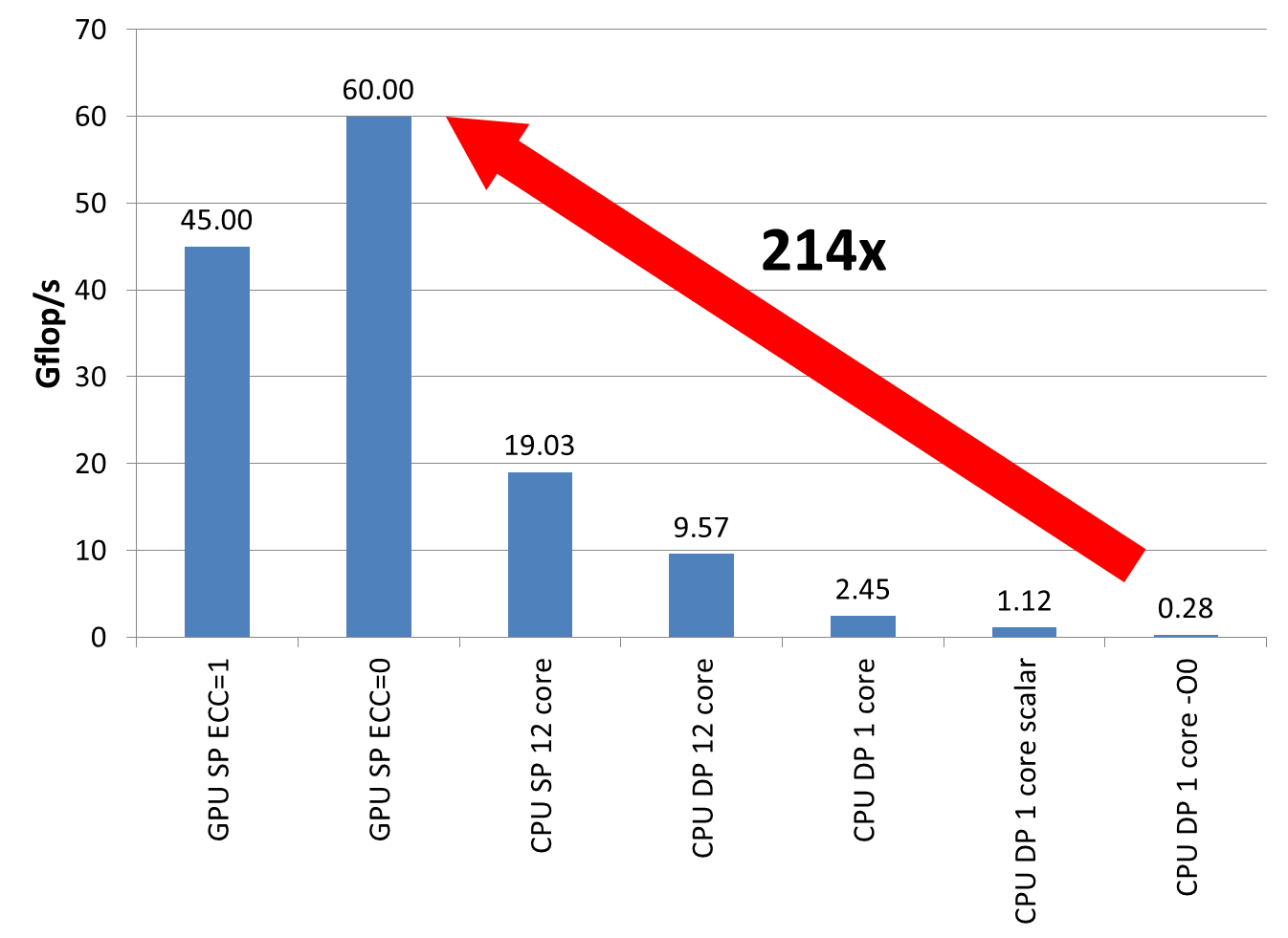
Figure 1: If you do it right, a 200x speedup for the GPU is absolutely feasible (comparing nVIDIA Tesla C2050 and Intel Dual Xeon 5650, dense matrix-vector multiply, matrix size 4500×4500, Intel compiler V12 update 11)
These tricks should give you a competitive edge; 20x-200x reported speedup should be no problem, depending on your unscrupulousness.
See Fig. 1 for an instructive example: A dense matrix-vector multiply using a 4500×4500 matrix is memory-bound on a Fermi-type GPGPU as well as on a standard CPU-based system such as a dual-socket Xeon 5650 (“Westmere”). The GPGPU baseline of about 45 GFlop/s at single precision (SP) is completely in line with the achievable memory bandwidth of roughly 90 GB/s (4 bytes per multiply-add operation, assuming the right-hand side is mostly held in shared memory). To get a slight speedup you can switch off ECC (who cares for some flipped bits?) to get about 120 GB/s, corresponding to 60 GFlop/s. No need to mention that the PCIe transfers to get the RHS and result vectors to and from the device are neglected. So much for the GPGPU.
On the CPU side, the full dual-Xeon node has a bandwidth of close to 40 GB/s, leading to an SP performance of 19 GFlop/s – much too fast to be shown in public! Going to double precision cuts that in half, but there is more: Using just a single core gets you down another factor of 4, and disabling vectorization gives you a further 0.5x (since you’re now far away from any bandwidth limitation). Finally, turning off optimization altogether (-O0) lets you hit rock bottom at 248 MFlop/s – a whopping 214x slower than the best GPGPU result! Going to my old P-III is not even necessary any more.
Note the cunning use of a linear scale in the diagram; in this particular case it is much better than a log scale since it reduces the CPU performance “baseline” to a mere flyspeck (see Stunt 3 for more information on log vs. linear scale).
This stunt is essentially identical to #6 and #7 of Bailey’s original collection.