Hello readers,

This is the second part from the 4-part CUDA-Aware-MPI series.

In this blog series, we will use only NVIDIA GPGPUs and assume that the user know basics about CUDA-Aware-MPI  from the official blogpost : https://developer.nvidia.com/blog/introduction-cuda-aware-mpi/[1]. Also, we assume that the reader knows about solving the 2D Poisson equation. For this, we are going to use a Jacobi solver on GPU.

Note: In CUDA-Aware-MPI, it is important to understand that MPI ranks only run on CPU. It is the MPI rank running on a particular CPU core that selects the GPU using:

cudaGetDeviceCount(&num_devices)    //Gets number of GPU device per node. 
cudaSetDevice(rank % num_devices)   //Particular MPI rank invoking this selects the GPU for execution

There are other relevant issues like the MPI rank selecting a GPU closest to the CPU-NUMA domain on which the MPI rank is pinned/tagged. But I do not wish to introduce those issues in this blog series. The reader can rest assured that these uncovered topics will not affect this 4-part series and I will use one specific example on MPI rank selecting different GPUs only for the purpose of understanding.

For the second post, we will focus on an application that requires communication. Solving 2D Poisson equation with Jacobi solver is a perfect application, that requires communication after each Jacobi solver iteration, to exchange ghost cells. This way, GPUs perform an iteration of Jacobi solver and then use CUDA-Aware-MPI to perform the halo exchange. Below is a demonstration of 1D domain decomposition, and the ghost cells exchange pattern:

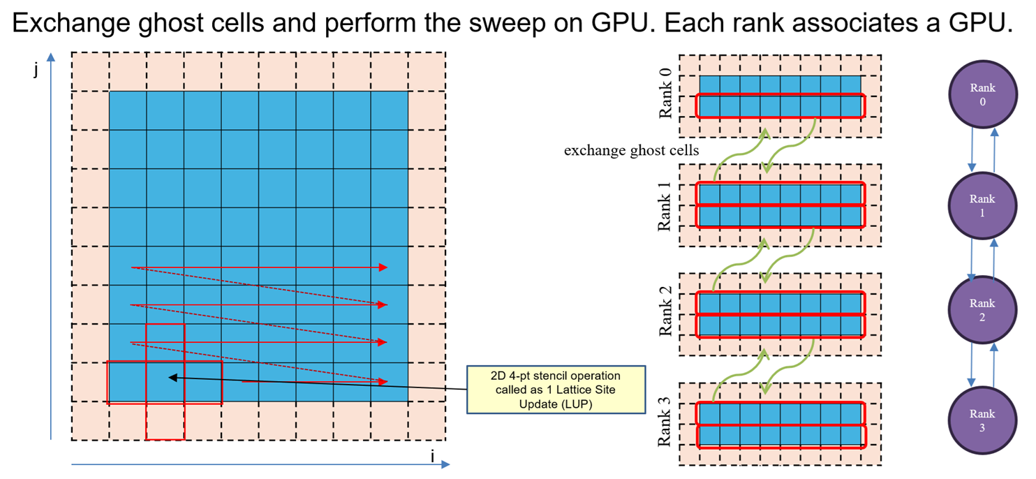
Explanation: 1 Jacobi operation requires top, bottom, left and right cells for computing, hence the name 2D 4-pt stencil. Each GPU performs 1 Jacobi iteration throughout their local domain. After performing 1 Jacobi iteration, the GPU need to exchange their cells on the boundary of their local domain,  so that each GPU can perform next Jacobi iteration. In the given example with 4 MPI ranks, you can see the communication pattern with 1D domain decomposition. Rank 0 and rank 3 has only 1 neighbor to exchange with, but rank 1 and rank 2 has to exchange with their top and bottom neighbors respectively to complete ghost cell exchange. Only then the GPUs can resume the next iteration of Jacobi. Here we use CUDA-Aware-MPI such that after each GPU completes 1 Jacobi iteration, it then performs ghost cell exchange with other GPUs, and then resume next iteration of Jacobi.

Note: This uses peer-to-peer communication method. So individual MPI_Isend and MPI_Irecv calls for each neighbor. Also note that we are performing 1D domain decomposition in j-direction. So we are communicating contiguous cells from each local domain. We will see the effects of communicating non-contiguous cells in the next part, when we move to 2D domain decomposition.

We now see the intranode scaling results for solving the 2D Poisson equation with 1D domain decomposition on all previous discussed nodes: A40, A100 and H100 nodes:

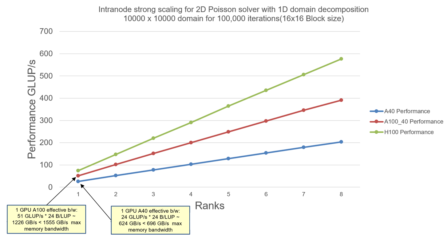
Explanation: We can see that the strong scaling for a domain size of 10K x 10K with 100,000 iteration scales well within 1 node for all different GPUs. The domain size for the problem is chosen such that the local domain stays out of cache. The number of iterations is chosen such that GPUs have enough work to do. The thread-block size is 16×16 (256 threads). Since Jacobi solver is memory-bound algorithm, we perform some Roofline analysis on the performance numbers. Single GPU performance is well within the memory bandwidth limit as seen in the picture above. As we increase more rank (1 GPU per rank) working on the same problem, we see no communication overheads. Hence the program will scale until GPUs do not have enough work (the local domain gets too small to saturate memory bandwidth and the local domain will fit into the GPU cache).

We now scale our program with 8 nodes (1 MPI process per node and 1 GPU per node):

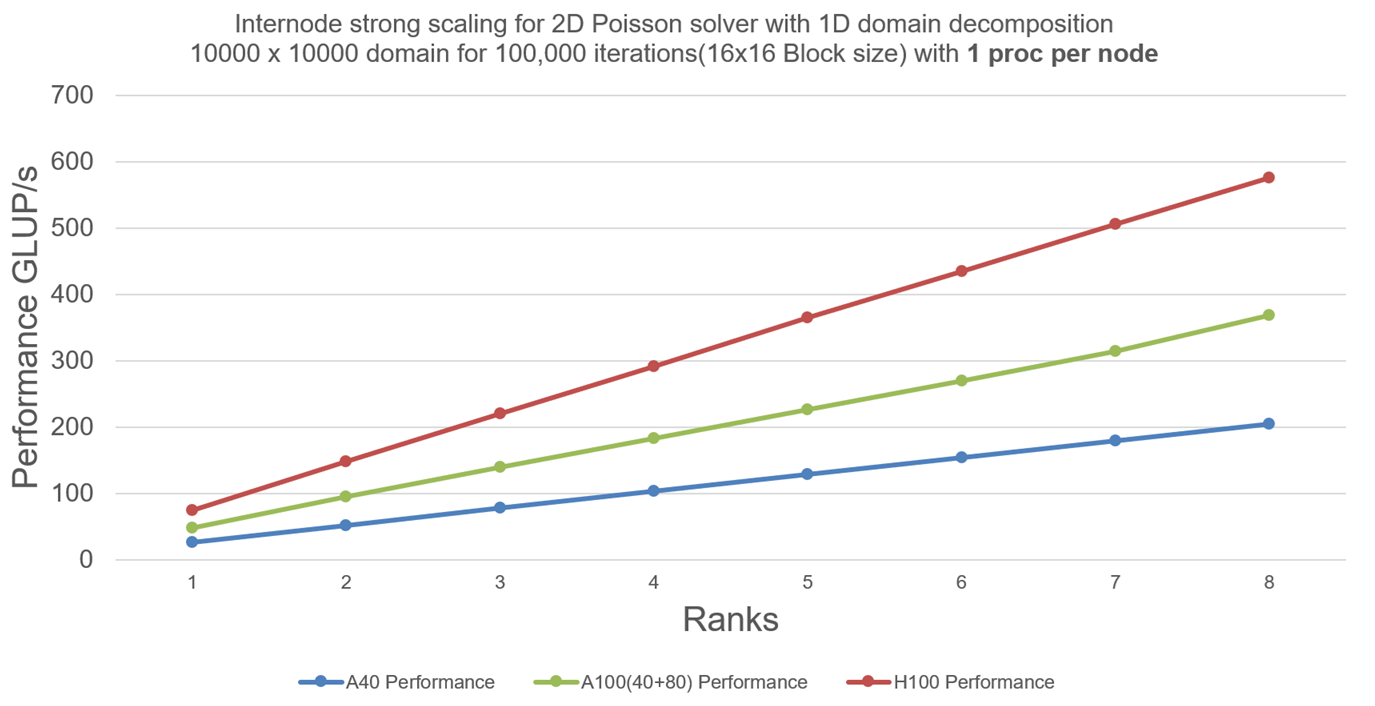
Explanation: We can still see that GPUs have enough work per Jacobi iteration and there is not much communication overhead from CUDA-Aware-MPI, hence scaling well with 8 nodes.

Now, how do the communication overhead looks like when there is not enough work for GPUs ? Lets take an interesting case with 5K x 5K domain size and perform internode strong scaling with 8 nodes (1 MPI process per node and 1 GPU per node):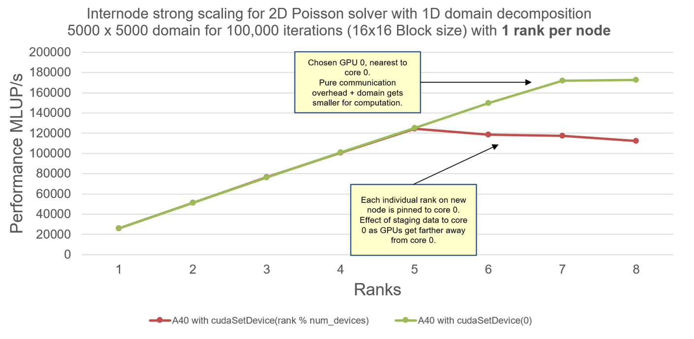

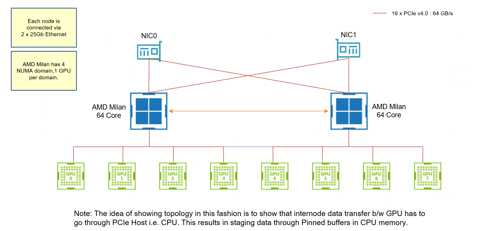
Explanation: In this example, we only look at A40 nodes. From the previous post, I should remind the reader that A40 nodes do not have GPUDirect RDMA drivers. Hence every CUDA-Aware-MPI communication between GPUs is actually stages through CPUs. Also, the reader is advised to revisit the topology of A40 nodes here.  5K x 5K is small enough domain such that the local domain gets smaller with increasing number of GPUs. Lastly, remember how I warned you before about the ability of MPI rank to select the GPU within the node ? We see the effects of a MPI rank selecting GPU farther from the CPU core, resulting in more time for staging the data when communicating.

Case 1: cudaSetDevice(0)  allows each MPI rank to select the first GPU within the node. I have deliberately pinned each MPI rank to the core 0 of the CPU on each node. So selecting GPU 0 nearest to the CPU is best option when data is staged during internode communication.

Case 2: cudaSetDevice(rank % num_devices) allows each MPI rank to select GPUs based on its own rank. Since there are 8 GPUs per node, and we are using 1 MPI rank per node across all 8 nodes, MPI ranks >= 5 will choose GPUs farther from core 0(we are again pinning each MPI rank to core 0 on each node). Hence requiring more time for staging the data (since the data has to travel from GPU 5, 6, 7, 8 to core 0, the far distance requires more time for staging). GPUs selected farther from the MPI rank always result in more communication time.

That is why understanding node topology is important. It also shows the essence of GPUDirect RDMA driver.

In the next part, we move on to the 2D Domain decomposition for solving the 2D Poisson equation. Same problem as above, but requires communication in both directions.

Thanks to NHR@FAU for letting me use their clusters for benchmarking.

For any questions regarding results or code, you can mail me at: aditya.ujeniya@fau.de