Hello readers,

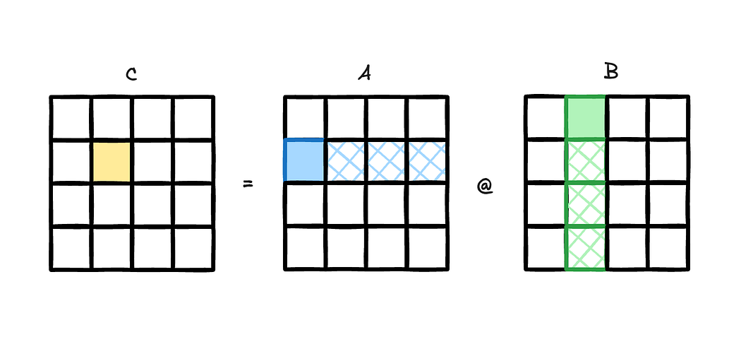
Today we talk about power and frequency characteristics of compute bound code, particularly SGEMM and DGEMM codes, but with a focus on different data initialization techniques. GEMMs are acronym for General Matrix Matrix multiplication. DGEMMs (Double-Precision GEMMs) involves 64 bit data (FP64 or double datatype) where it uses input matrix of FP64 datatype  and computes GEMM in an output matrix of FP64 datatype. On the other hand, SGEMMs (Single-Precision GEMMs) involves 32 bit data (FP32 or float datatype) where it uses input matrix of FP32 datatype  and computes GEMM in an output matrix of FP32 datatype. Below is a simple diagram[fig] to understand 2D GEMM intuitively.

It is not in this post’s intension to explain GEMM or optimization techniques. We assume the reader knows about GEMM and also about CuBLAS library. The DGEMM benchmark used can be found here and SGEMM benchmark used can be found here. They use direct CuBLAS calls to cublasDgemm and cublasSgemm functions. We use 2D matrices instead of 3D matrices, which still fulfill our goal. Our goal is to reach peak performance of the GPUs and compute bound codes are the best way to do it. Reaching peak performance usually mean using almost all compute units, which then activates most of the transistors, resulting in more power consumption.

We will explore power and frequency characteristics for 3 different types of data initialization. By data initialization, we mean initializing the input matrix A and B. For data initialization, we wrote a basic GPU kernel that initializes the data, rather than initializing on CPU and copying over to GPU. Below are the 3 cases for data initialization:

Case 1:

// Generate random numbers between 0 and 1
A[idx] = curand_uniform(&state);
B[idx] = curand_uniform(&state);
C[idx] = 0.0;

Case 2:

// Assign value of index
A[idx] = idx;
B[idx] = idx;
C[idx] = 0.0;

Case 3:

// Assign the whole matrix with 1 constant
A[idx] = 65.045;
B[idx] = 12.957;
C[idx] = 0.0;

For SGEMM data initialization, we just typecasted the doubles to float. You can have a look into the reference code given above.

We benchmarked these 3 cases on 3 different GPUs – NVIDIA A40, A100 and H100. A40 and A100 have Ampere Architecture and H100 has Hopper architecture. When we performed SGEMM and DGEMM on these 3 GPUs with 3 different data initialization techniques, we found something interesting.

Scenario 1: Benchmarking SGEMM on A40 

As we said earlier, we want to activate as much compute units as possible and reach the TDP of GPU. NVIDIA A40 has a TDP of 300W and it has 64x more FP32 compute units than FP64. Hence we use SGEMM on A40. When we performed SGEMM for a problem size of 54016² for 1000 iterations, we found some interesting results. The square matrix size of 54016² occupies 12 GB per matrix. In total the problem size is 36 GB for 3 matrices (A, B and C). This problem size is big enough to be called compute-bound problem size. Lastly, the Peak FP32 (non-Tensor) performance on A40 is 37.4 TFlop/s [ref]. Now, let us see the results for SGEMM with 3 different data initialization cases we talked about earlier:

Now we see SGEMM achieved performance is far away from A40 FP32 peak performance of 37 TFlop/s. We saw SM Throughput of 85% in NVIDIA compute reports. We should have observed 31.5 TFlop/s. The rest of the performance gap is observed because of frequency downscaling. The reason why we see frequency downscaling is because of power limit. Since this is compute bound code, most of the FP32 units are active and its draws max GPU power. Its obvious that when GPUs reach power limit (300W in case of A40), the temperature increases. To keep temperature within limits, the GPU downscales its SM frequency. Hence we see frequency suppression or downscaling. Another term for frequency downscaling is called “throttling”.  Throttling is the process of slowing down(by reducing frequency) your CPU/GPU in order to reduce heat and power use.

What’s interesting here is that we see difference in performance based on how your matrix data is initialized. Random data initialization offers the lowest, then linear matrix data is a bit better and constant matrix data is best of the all. Its obvious we see a performance difference due to different average frequency. The SM frequency seen in the graph above is the SM average frequency over time (means performing SGEMM for a given number of iterations and given problem size). The code where random data were initialized runs overall slower because for the whole problem, it performs SGEMM at lower frequency. On the other hand, code where constant data was initialized runs fastest of the three because it performs SGEMM at a better frequency over time. But what could be the reason that SGEMM with constant data initialization runs faster than SGEMM with random data initialization ?? The problem size and number of iterations is the same.  Other things we confirmed(from NVIDIA compute reports) that were exactly same between these 3 data initialization cases:

1. Thread block size: 256
2. 1 Thread block per SM –  kernel limited by 202 registers per thread
3. o% L1 cache hit rate
4. Same SM Throughput: 85 %
5. Same power draw: 300W
6. No data compression in L2 hierarchy
7. ECC was off

To find the mystery behind difference in frequency, my colleague S. Kuckuk asked me to check the data transfer in memory hierarchy. Below is the amount of data transferred during SGEMM with 3 different cases and the DRAM Throughput % (the amount of sustained memory bandwidth from the total memory bandwidth).

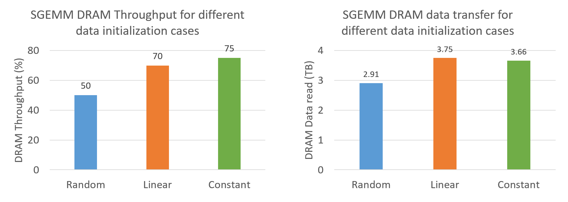
Now it gets more confusing because random data initialization case has the lowest DRAM Throughput as well as the amount of data transferred compared to linear and constant data initialization case. Its a bit counterintuitive since this could not be the reason for difference in performance.  Higher data transfer + higher DRAM Throughput does not result in higher SM frequency. The only reason we see this increase in data transfer could be due to how thread scheduling works at different frequency. Random data initialization case, which performs SGEMM at lower frequency, would allow threads to reuse data from L2, which then lead to request less data from DRAM. Linear and Constant data initialization case, which runs at higher SM frequency, would have a lower L2 hit rate because of threads not able to find data for reuse in L2 cache, hence requesting more data from DRAM to L2. To confirm this theory, we ran DGEMM on A100 with 3 data initialization cases.

Scenario 2: Benchmarking DGEMM on A100 

NVIDIA A100 can reach TDP of 400W with DGEMM benchmark. A100 has FP64 compute units as well as FP64 tensor cores units called TF64 or TP64. CuBLAS DGEMM usually operates on tensor cores (if present in NVIDIA GPUs), so our experiments will be on TP64. Peak TP64 performance for A100 is 19.5 TFlop/s [ref]. Below are the graphs that show a sweep over different DGEMM sizes for 3 different data initialization.

In these graphs, we can clearly see the effects of different data initialization cases. We see there is no throttling despite the fact that random data initialization cases reaches full TDP. This is good because all the 3 cases have average SM frequency of 1410 MHz. When we analyzed the NVIDIA Compute reports, we could see same data transfer from DRAM to L2 and same L2 % hit rate. This confirms our theory of how SMs operating at different frequency can lead to different L2 % hit rate, which then changes the DRAM data transfer amount. Lets get back to the A100 results. Since all the 3 data initialization cases reach peak TP64 performance with no frequency downscaling, its evident that data initialization has a major influence on power consumption. But why is there even a difference in power consumption based on how you initialize your matrix data ?? Everything is same –  the amount of threads per block, the amount of data transfer, the average SM frequency, the CuBLAS algorithm. Then what changes ??

The only reason we see such behaviors could be due to bit-flips while computing. Compute units performs bit manipulation in order to perform arithmetic operations. How many bits and transistors are active or how many bits were flipped while computing could be a major contributing factor to power consumption. In random data initialization case, within the 64 bits of each element, all the 64 bits are randomly active. Whereas in constant data initialization case, all the 64 bits are identical. This could happen during computation in order to save power consumption when less bit-flips are required. Let us see behavior of different data initialization on H100.

Scenario 3: Benchmarking DGEMM on H100 SXM

If we apply what we observed and learned from last 2 scenarios, we can easily infer from the graphs for H100. The peak TP64 or TF64 performance on H100 is 67 TFlop/s [ref]. NVIDIA H100 SXM  has a TDP of  700W, although in the graphs you see limit of 500W. Our H100 is power capped at 500W.

We observe frequency downscaling or throttling again. For a sweep of different matrix sizes, we see difference in performance for 3 different data initialization cases. Random data case, as we know will have lowest performance compared to constant data case, which should have the highest performance.

Conclusion for compute-bound codes on NVIDIA GPUs

1. If the GPU is throttling, we should see difference in performance based on how your input matrices are initialized.
2. If the GPU is not throttling, we should see difference in power consumption based on how your input matrices are initialized.
3. For a same problem size, difference in SM frequency changes the amount of data transfer, due to the different L2 cache hit rate.

Thanks to NHR@FAU for letting me use their clusters for benchmarking.

For any questions regarding results or code, you can mail me at: aditya.ujeniya@fau.de