Hello readers,

This is the fourth part from the 4-part CUDA-Aware-MPI series.

In this blog series, we will use only NVIDIA GPGPUs and assume that the user know basics about CUDA-Aware-MPI  from the official blogpost : https://developer.nvidia.com/blog/introduction-cuda-aware-mpi/[1]. Also, we assume that the reader knows about solving the 2D Poisson equation. For this, we are going to use a Jacobi solver on GPU.

In the part 2 and part 3 of this series, we used a specific application of solving the 2D Poisson equation with 1D and 2D domain decomposition. We performed strong scaling with intranode and internode setups. There was no problem when scaling the application/program with 1D domain decomposition, but it was way more worse when scaling the program with 2D domain decomposition. The reason for worse performance: when GPUs want to communicate strided elements to other GPU using CUDA-Aware-MPI, then GPUs will stage every strided element to CPU memory and then communicate, since packing of strided elements has to be done first into contiguous buffer. We want to circumvent this method by introducing custom packing kernels.

Idea: Instead of depending on CUDA-Aware-MPI to stage and pack in CPU memory, we introduce our own kernels that performs packing in GPU memory. The packing will be done by collecting strided elements into a contiguous buffer in GPU memory itself. Since we are using 2D domain decomposition, it involved exchanging ghost cells with top/bottom/left/right neighbors. Top/bottom ghost cell exchange is not a problem because the elements are contiguous in GPU memory. Left/right neighbors ghost cell exchange require packed strided elements, which we will now pack and unpack using GPUs themselves.

So the process of optimizing 2D domain decompos

• Step 1. Use GPUs to pack data from strided memory location into contiguous buffers into GPU memory for left/right neighbors.
• Step 2. Overlap computation/packing from step 1 with communication with top/bottom neighbors using cuda_stream.
• Step 3. Before sending the packed data to left/right neighbors, sync the cuda_stream and then send the packed buffers.
• Step 4. Use GPUs to again unpack from the received contiguous buffers back to strided memory locations in the GPU memory.

A simple pseudocode looks like this:

void exchange_device(cudaStream_t copyStream)

{

    const int blockSize = 1024;

    const int gridSize = 1 + (jLocal + 2) /  blockSize;

    // For LEFT and RIGHT neighbours, let GPUs pack into contiguous buffers.
    copy_edge_to_block<<<gridSize, blockSize, 0, copyStream>>>(LEFT; RIGHT);

    // Can overlap GPU computation with GPU communication to TOP and BOTTOM neighbors.
    simple_exchange(TOP; BOTTOM);

    // Synchronize cuda_stream before sending the data to LEFT and RIGHT neighbors.
    cudaErrorCheck(cudaStreamSynchronize(copyStream));

    // Exchange with LEFT and RIGHT neighbors
    simple_exchange(LEFT; RIGHT);

    // Use GPUs to copy back the data from contiguous buffers to strided memory locations.
    copy_block_to_edge<<<gridSize, blockSize, 0, copyStream>>>(LEFT; RIGHT);

}

 

copy_edge_to_block<<<>>> kernel will copy from strided memory locations into one contiguous buffer in GPU memory. We call this packing operation as computation.

copy_block_to_edge<<<>>> kernel will copy from the received contiguous buffer into the strided memory locations n GPU memory.

Now that we have implemented an optimized 2D domain decomposition, we can compare it with 1D domain decomposition. Below I compare the results for internode strong scaling for 10K x 10K domain size for 100,000 iterations. Again the setup for internode scaling is 1 MPI process per node and 1 GPU per node.

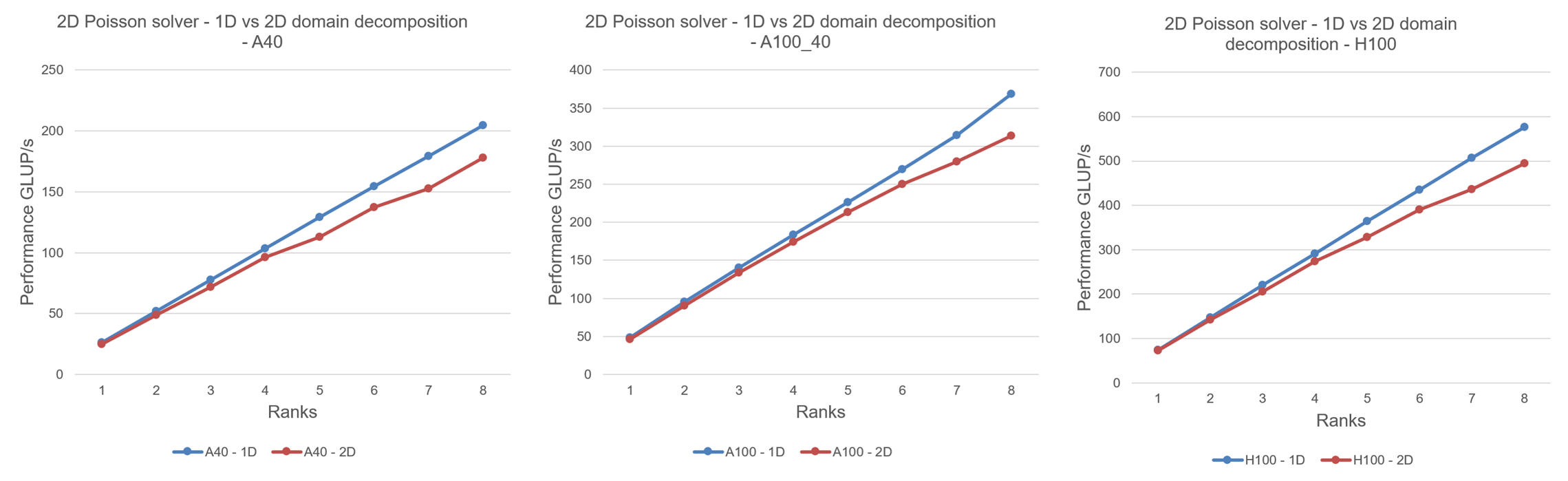
Explanation: As know from previous posts, we know that program with 1D domain decomposition scales well and linearly until pure communication overheads starts to come into play. For program with optimized 2D domain decomposition, we see that there are overheads, but these overheads are not from pure communication, but something else. The observed overhead in 2D domain decomposition is from packing/unpacking on GPUs, resulting into less performance as compared with 1D domain decomposition. It does not scale linearly, but atleast it scales well than the performance seen in part 3. Performance drops are highly seen with prime number of MPI ranks because the 2D domain decomposition cannot distribute prime numbers in both dimensions. So the 2D domain decomposition happens in only 1 dimension for prime number of MPI ranks. Because the 2D domain decomposition for prime number happens only in i-direction/x-direction, for all ranks, there is only left and right neighbor for ghost cells exchange. The GPUs do not have any top/bottom neighbor and there is no overlap of computation/communication. Otherwise, where there are more top/bottom neighbors with left/right neighbors, the GPUs can overlap computation/communication.

This idea of optimizing 2D domain decomposition was derived from the original NVIDIA blogpost: https://developer.nvidia.com/blog/benchmarking-cuda-aware-mpi/

I hope you have enjoyed reading this series and learned something new. There is also some work done by Carl Pearson on optimizing the packing/unpacking of the strided/contiguous elements in CUDA-Aware-MPI. He has written a custom kernel adaptable to various stride lengths and Grid+Block configurations. You can find his study here: https://carlpearson.net/post/20201006-mpi-pack/

Thanks to NHR@FAU for letting me use their clusters for benchmarking.

For any questions regarding results or code, you can mail me at: aditya.ujeniya@fau.de