(See the prelude for some general information about what this is all about)
As we have seen in Stunt 2 about slowing down code execution, making all parts in the speedup formula except communication overhead more dominant is good for the straightness of your scalability graph. Weak scaling, i.e., keeping the problem size per worker constant while increasing the number of workers, is probably the simplest way to achieve this (\alpha=1 in the speedup formula). Neglecting boundary effects, many codes will then show a constant ratio of communication overhead versus computation time; given a reasonably nonblocking network hierarchy, linear scalability often comes for free, at least for a large enough number of nodes. A positive side effect is that you don’t even have to recompile, let alone change your code.You can then even show real performance numbers, not just speedups!

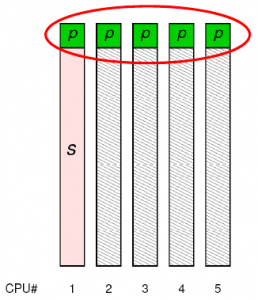
Fig. 1: Weak scaling with a dominating serial part. The scalability function has a small slope, but the “work” done in the parallel part scales perfectly.
In case there is no communication problem but a large serial part, just by choosing the right metric to look at you can get perfect scaling, i.e., S(N)=N. Here’s how it works: Let’s assume that, despite weak scaling, your code is dominated by a sequential part. Hence, it’s S(N)=s+(1-s)N. The function is linear but has a small slope, which doesn’t look good and leads to a parallel efficiency \varepsilon(N)=S(N)/N that is much smaller than 1. However, looking at how the processors spend their time it is clear that the speedup function for the purely parallel work per time unit, i.e., not counting any overhead, is linear in N with a slope of 1 (see Fig. 1). How can this be used to polish performance numbers? Just report a performance metric that is valid only for the purely parallel part of the application! MFlop/s or MLup/s (lattice site updates) will do fine, for instance. If the “overhead” part contains no lattice updates, the MLup/s metric has a perfect speedup function S_\mathrm{mlups}(N)=N, the performance graph is linear with no y-intercept, and \varepsilon(N)=1, even though all but one processor are twiddling their thumbs most of the time. Problem solved. Stay tuned for Stunt 10, where we will show that a similar trick is possible for communication-dominated cases as well.
The reason why it works is that we have chosen a different notion of what “work” means in the speedup formula. Speedup is defined as
S(N)=\frac{\text{work/time with \textit{N} workers}}{\text{work/time with 1 worker}}~,no matter whether the amount of work varies with N or not. While there is no discussion about what “time” means, we can give different meanings to “work”. If “work” is chosen so that only operations in the parallel part are counted, parallel efficiency is perfect at weak scaling (\alpha=1). That trick cannot be pulled at strong scaling, though (it is left to the reader to prove this…).
It is certainly advisable to omit any mention of the fact that weak scaling was used. Your audience will cheer and rejoice in the light of such straight lines! However, don’t let them watch too long or they’ll ask nasty questions…
This stunt is essentially #4 of Bailey’s original “Twelve ways to fool the masses.”