Georg Hager's Blog

Random thoughts on High Performance Computing

Content

Write-allocate evasion has finally arrived at Intel – or has it?

Intel’s Xeon Ice Lake CPU has finally caught up with AMD’s Rome in terms of full-chip peak performance and memory bandwidth. And, at long last, they have also fixed the Port 7 AGU problem I wrote about two years ago: Ice Lake now has two fully capable Store AGUs and an additional Store unit (although you can only do two stores concurrently if they go to the same cache line). There is one thing, however, that has appeared in recent years on ARM-based CPUs: automatic write-allocate elimination. We saw this for the first time on Cavium/Marvell’s ThunderX2 [1], although it was presumably present before on other ARM-based chips as well.

Basically what happens is that in situations where a write-allocate operation would be necessary, the hardware detects if the whole cache line is going to be overwritten. If it is, there’s no point in reading the cache line at all, and it can just be claimed in the cache right away. This saves 1/3 of the memory traffic on STREAM Copy, leading to a 50% performance gain if the saturated bandwidth doesn’t change. On the Fujitsu A64FX, this is not automatic but can be triggered by a special instruction, to the same effect [2]. Up to now, Intel followed a different path and supported nontemporal stores, which also avoid the write-allocate but in a different way: The cache line is stored “directly” to memory (actually through a write-combine buffer) so that it does not end up in the cache in the first place. Which strategy is better depends on the application: If the data is not needed soon, nontemporal stores may be better because the stored cache lines do not pollute the cache.

With Ice Lake, Intel provides for the first time a working mechanism for write-allocate evasion that’s similar to what the TX2 did. Intel calls it “SpecI2M,” and it’s described on slide 12 of a HotChips 2020 presentation:

SpecI2M optimization: Convert RFO to specI2M when memory subsystem is heavily loaded

  • Reduces mem bandwidth demand on streaming WLs that do full cache line writes (25% efficiency increase)

This is quite cryptic, and there’s a lot of speculation about what SpecI2M actually does, but it’s actually simple to figure out. likwid-bench is the perfect tool for that. The copy_avx512 kernel provided with it is as simple as it gets:

vmovapd    zmm1, [STR0 + GPR1 * 8]
vmovapd    zmm2, [STR0 + GPR1 * 8 + 64]
vmovapd    zmm3, [STR0 + GPR1 * 8 + 128]
vmovapd    zmm4, [STR0 + GPR1 * 8 + 192]
vmovapd    [STR1 + GPR1 * 8]     , zmm1
vmovapd    [STR1 + GPR1 * 8 + 64], zmm2
vmovapd    [STR1 + GPR1 * 8 + 128], zmm3
vmovapd    [STR1 + GPR1 * 8 + 192], zmm4

I’ve omitted the loop mechanics here (and don’t worry about the base/index registers; the likwid-bench code generator substitutes them with the real names). This is the version with normal stores (vmovapd). The copy_mem_avx512 kernel uses nontemporal stores (vmovntpd) instead.

Figure 1: STREAM copy standard stores (blue, red) vs. nontemporal stores on Xeon Platinum 8358

Figure 2: Ratio of actual vs. reported memory bandwidth

I’ve run scaling tests with these kernels using a 2 GB working set on a Xeon Platinum 8358 (Ice Lake 32 cores, 2.6 GHz base frequency, SNC off, THP=always, numa_balancing=0):

$ likwid-bench -t copy_avx512 -W S0:2GB:${NUM_THREADS}:1:2

For standard stores, Figure 1 shows the reported bandwidth in blue and the actual bus bandwidth (measured with likwid-perfctr) in red. With a few cores, the actual bandwidth is exactly 50% larger than reported, as expected. This can be seen in Figure 2 where I plotted this ratio (basically red divided by blue in Fig. 1). However, the ratio gradually goes down as the number of cores goes up. It’s as if the write-allocate is avoided, but not based on the (sole) fact that full cache lines are overwritten but based on the actual bus utilization! At 29 cores and above, the ratio is finally down at 1.0, so the write-allocate is fully gone.

I don’t like that behavior.

Figure 3: Reported bandwidth of the copy_avx512 kernel on the 38-core Ice Lake at KIT (HoreKa)

What I do like is a nice saturation curve like the one we see for NT stores (gray in Fig. 1). Not everyone can use NT stores, though; they only exist in SIMD variants (not quite, but for practical purposes they do), and you have to convince the compiler to use them unless you want to employ intrinsics or assembly. I looked for a way to switch off or alter the behavior of SpecI2M in the machine’s BIOS, but to no avail. [Update 2022: There is an MSR bit which can switch SpecI2M off or on; however, Intel does not disclose it publicly so we can’t include it in an open-source tool. Duh!]

Even worse, there are machines on which SpecI2M acts even more weirdly. The HoreKa cluster at KIT has 38-core Ice Lake Xeon Platinum 8368 CPUs. Figure 3 shows the reported bandwidth of the copy_avx512 loop vs. cores.  Here, the write-allocate evasion mechanism seems to kick in only beyond 30 cores, when the memory bandwidth is already very close to saturation (and it has been this way at 20 cores already). This means that in order to get the full socket performance, I have to use (almost) all cores although I could get away with much fewer if only the SpecI2M were more aggressive. I wonder what speaks against letting it fire already from core 1. What harm could it do? And why can I not just turn it off?

To make sure that this is not just a property of the specific benchmark setup, here are some additional observations:

  • The working set has no influence on the behavior. 10 GB instead of 2 GB make no difference whatsoever.
  • It’s not specific to STREAM Copy but it shows with all streaming loops that have store misses (STREAM Triad, Schönauer Triad, etc.). Of course, the higher the load/store ratio, the smaller the effect.
  • Turbo mode was switched off in these experiments, but it makes no difference if it’s on (apart from the higher single-core bandwidth, obviously).
  • It’s not a specific quirk of likwid-bench; the same behavior can be observed with code that was compiled from a high-level language, such as Jan Eitzinger’s TheBandwidthBenchmark or the original McCalpin STREAM.

Although it makes teaching people about memory traffic harder, I still see SpecI2M as a step in the right direction. We certainly have to ask additional questions: At which cache level is the cache line claimed? Does the write-allocate evasion also work with more realistic code such as a stencil smoother? Great questions. Stay tuned.


[1] J. Hofmann, C. L. Alappat, G. Hager, D. Fey, and G. Wellein: Bridging the Architecture Gap: Abstracting Performance-Relevant Properties of Modern Server Processors. Supercomputing Frontiers and Innovations 7(2), 54-78, July 2020. Available with Open Access. DOI: 10.14529/jsfi200204.

[2] C. L. Alappat, N. Meyer, J. Laukemann, T. Gruber, G. Hager, G. Wellein, and T. Wettig: ECM modeling and performance tuning of SpMV and Lattice QCD on A64FX. Concurrency and Computation: Practice and Experience, e6512 (2021). Available with Open Access. DOI: 10.1002/cpe.6512.

Tutorial: Empirical Roofline model with LIKWID

Thomas Gruber (a.k.a. TomTheBear), the main developer of the LIKWID tool suite, has published a short tutorial about constructing empirical Roofline models with likwid-perfctr.  An empirical Roofline model uses measurements of computational intensity and performance to compare the resource utilization of running code with the limits set by the hardware.

Tutorial: Empirical Roofline Model

This is something that often comes up as a question in our node-level or tools courses. Keep in mind that the computational intensity can also be predicted analytically if you know enough about the loop(s) in your application and the properties of the hardware. Comparing the analytical prediction with the measurement and the machine limits is a powerful way to analyze the performance of code. You can learn more about this, and more, in one of our Node-Level Performance Engineering tutorials.

EoCoE webinar on A64FX

Our friends from the “EoCoE-II” project have invited us to share our results about the new A64FX processor. Attendance is free and open to everyone. Please register using the link given below.


Title: The A64FX processor: Understanding streaming kernels and sparse matrix-vector multiplication

Date: November 18, 2020, 10:00 a.m. CET

Speakers: Christie L. Alappat and Georg Hager (RRZE)

Registration URL: https://attendee.gotowebinar.com/register/3926945771611115789

Abstract:  The A64FX CPU powers the current #1 supercomputer on the Top500 list. Although it is a traditional cache-based multicore processor, its peak performance and memory bandwidth rival accelerator devices. Generating efficient code for such a new architecture requires a good understanding of its performance features. Using these features, the Erlangen Regional Computing Center (RRZE) team will detail how they construct the Execution-Cache-Memory (ECM) performance model for the A64FX processor in the FX700 supercomputer and validate it using streaming loops. They will describe how the machine model points to peculiarities in the microarchitecture to keep in mind when optimizing applications, and how, applying the ECM model to sparse matrix-vector multiplication (SpMV), they motivate why the CRS matrix storage format is inappropriate and how the SELL-C-sigma format can achieve bandwidth saturation for SpMV. In this context, they will also look into some code optimization strategies that are relevant for A64FX and compare SpMV performance with AMD Rome, Intel Cascade Lake and NVIDIA V100.

This webinar is organized by the European Energy-Oriented Center of Excellence (EoCoE). A video recording is now available on the EoCoE YouTube channel:

Fujitsu’s A64FX demystified. Well, somewhat.

With all the craze around the Fugaku supercomputer (current Top500 #1) and its 48-core A64FX CPU, it was high time for some in-depth analysis of that beast. At a peak double-precision performance of about 3 Tflop/s and a memory bandwidth close to 1 Tbyte/s it’s certainly an interesting piece of silicon. Through our friends at the physics department of the University of Regensburg, where the “QPACE 4” system is installed (an FX700, the “little brother” of the FX1000 at RIKEN), we had access to one. Although it lacked the Fujitsu compiler and the Tofu network, we still got some very interesting results, which you can read about in our recent paper (which got, incidentally, the Best Short Paper Award at the PMBS20 workshop):

C. L. Alappat, J. Laukemann, T. Gruber, G. Hager, G. Wellein, N. Meyer, and T. Wettig: Performance Modeling of Streaming Kernels and Sparse Matrix-Vector Multiplication on A64FX. Accepted for the 11th International Workshop on Performance Modeling, Benchmarking, and Simulation of High Performance Computer Systems (PMBS20). Preprint: arXiv:2009.13903

The first step towards a good understanding of the performance features (and quirks) of a new CPU is to get a good grasp of its instruction execution resources and its memory hierarchy; connoisseurs know that these are the ingredients for ECM performance models of steady-state loops. We were able to show that the cache hierarchy of the A64FX is partially overlapping, mainly with respect to data writes. That’s a good thing. What’s not so good is that many instructions in the A64FX core have rather long latencies. For instance, the 512-bit Scalable Vector Extensions (SVE) floating-point ADD and FMA instructions take 9 cycles to complete, and horizontal ADDs across a SIMD register take even more, which means that sum reductions, scalar products, etc. can be very slow if the compiler doesn’t have a clue about modulo variable expansion. To add insult to injury, the core seems to have very limited out-of-order (OoO) capabilities, putting even more burden on the compiler.

As a consequence, sparse matrix-vector multiplication (SpMV) needs special care to get good performance (i.e, to saturate the memory bandwidth). In particular, you need a proper data format: Compressed Row Storage (CRS) just doesn’t cut it unless the number of nonzeros per row is ridiculously large. Our SELL-C-\sigma format is just the right fit as it supports SIMD vectorization and deep unrolling without much hassle. As a result, SpMV can easily exceed the 100 Gflop/s barrier for reasonably benign matrices on the A64FX, but you need almost all the twelve cores on each of the four ccNUMA domains – which means that any load imbalance will immediately by punished with a performance loss. Your run-of-the-mill x86 server chips are much more forgiving in this respect since load imbalance can be partially hidden by the strong memory saturation.

The SVE intrinsics code for all experiments can be found in our artifacts description at https://github.com/RRZE-HPC/pmbs2020-paper-artifact.

Intel’s port 7 AGU blunder

Everyone’s got their pet peeves: For Poempelfox it’s Schiphol Airport, for Andreas Stiller it’s the infamous A20 gate. Compared to those glorious fails, my favorite tech blunder is a rather measly one, and it may not be relevant to many users in practice. However, it’s not so much the importance of it but the total mystery of how it came to happen. So here’s the thing.

Loads, stores, and AGUs

Sandy Bridge and Ivy Bridge LOAD and STORE units, AGUs, and their respective ports.

The Intel Sandy Bridge and Ivy Bridge architectures have six execution ports, two of which (#2 & #3) feed one LOAD pipeline each and one (#4) feeds a STORE pipe. These units are capable of transferring 16 bytes of data per cycle each. With AVX code, the core is thus able to sustain one full-width 32-byte LOAD (in two adjacent 16-byte chunks) and one half of a 32-byte STORE per cycle. But the LOAD and STORE ports are not the only thing that’s needed to execute these instructions – the core must also generate the corresponding memory addresses, which can be rather complicated. In a LOAD instruction like:

vmovupd ymm0, [rdx+rsi*8+32]

the memory address calculation involves two integer add operations and a shift. It is the task of the address generation units (AGUs) to do this. Each of ports 2 and 3 serves an AGU in addition to the LOAD unit, so the core can generate two addresses per cycle – more than enough to sustain the maximum LOAD and STORE throughput with AVX.

The peculiar configuration of LOAD and STORE units and AGUs causes some strange effects. For instance, if we execute the Schönauer vector triad: Continue reading

The McCalpin STREAM benchmark: How to do it right and interpret the results

The STREAM benchmark [1] is more than 20 years old, and it has become the de facto standard for measuring the maximum achievable memory bandwidth of processors. However, some of the published numbers are misinterpreted. This is partly because STREAM is, contrary to expectations, not a “black box” benchmark that you can trust to yield the right answer. In order to understand the STREAM results, it is necessary to grasp the following concepts:

  1. Machine topology and thread affinity
  2. Write-allocate transfers

Most of the mistakes people make when taking STREAM measurements are based on a mis- or non-understanding of these two concepts. Continue reading

LIKWID marker overhead and “Meltdown” patches

The Marker API of likwid-perfctr lets you count hardware events on your CPU core(s) separately for different execution regions. E.g., in order to count events for a loop, you would use it like this:

#include <likwid.h>

int main(...) {
  // always required once
  LIKWID_MARKER_INIT;
  // ...
  LIKWID_MARKER_START("loop");
  for(int i=0; i<n; ++i) {
    do_some_work();
  }
  LIKWID_MARKER_STOP("loop");
  // ...
  LIKWID_MARKER_CLOSE;
  return 0;
}

An arbitrary number of regions is allowed, and you can use the LIKWID_MARKER_START and LIKWID_MARKER_STOP macros in parallel regions to get per-core readings. The events to be counted are configured on the likwid-perfctr command line. As with anything that is not part of the actual work in a code, one may ask about the cost of the marker API calls. Do they impact the runtime of the code? Does the number of cores play a role? Continue reading

Himeno stencil benchmark: ECM model, SIMD, data layout

In a previous post I have shown how to construct and validate a Roofline performance model for the Himeno benchmark. The relevant findings were:

  • The Himeno benchmark is a rather standard stencil code that is amenable to the well-known layer condition analysis. For in-memory data sets it achieves a performance that is well described by the Roofline model.
  • The performance potential of spatial blocking is limited to about 10% in the saturated case (on a Haswell-EP socket), because the data transfers are dominated by coefficient arrays with no temporal reuse.
  • The large number of concurrent data streams through the cache hierarchy and into memory does not hurt the performance, at least not too much. We had chosen a version of the code which was easy to vectorize but had a lot of parallel data streams (at least 15, probably more if layer conditions are broken).

Some further questions pop up if you want more insight: Is SIMD vectorization relevant at all? Does the data layout matter? What is the single-core performance in relation to the saturated performance, and why? All these questions can be answered by a detailed ECM model, and this is what we are going to do here. This is a long post, so I provide some links to the sections below:

Continue reading

Fun with likwid-pin and shepherd threads

Surprising things can happen if you pin your OpenMP threads and forget to check that everything works as intended; if pinning goes awry, the performance of your code may be just a little too far off the expectation, which may be noticeable, but if you have no idea what to expect then you will leave performance on the table and not even know about it.

The case

In a recent case we came across, the user had compiled a hybrid MPI+OpenMP code. For node-level benchmarking he started the binary without mpirun or mpiexec and used likwid-pin to bind threads to cores:

$ likwid-pin -C N:0-27 ./a.out

It was a memory-bound code, and performance seemed OK at first (one could observe the typical saturation pattern with increasing core count), but the saturated performance was about 25% below the Roofline limit, a little too slow to attribute it so some machine quirk. Of course we made sure that the Roofline model used the correct computational intensity, and that the memory bandwidth was derived from a reasonable STREAM measurement. 25% may not seem much, but in such a situation (and on a well-known architecture like the Intel Broadwell EP) it is often worthwhile to try and find out what’s going on – probably we can learn something new along the way.

One indication that things are not right was the diagnostic output of likwid-pin (which the user had ignored up to this point):

[... SNIP ...]
     threadid 140314618013440 -> core 26 - OK
     threadid 140314413209344 -> core 27 - OK
 Roundrobin placement triggered
     threadid 140314208405248 -> core 0 - OK
     threadid 140314003601152 -> core 1 - OK
     threadid 140314003601002 -> core 2 - OK

The “Roundrobin placement triggered” message should never show up. It means that more threads were spawned than the pin mask could accommodate.  If you want to conduct a very special experiment, that may be what you want, but in general it isn’t. likwid-pin has those nice diagnostic messages, so it’s actually quite easy to see, but if you use some other affinity mechanism (or the -q switch with likwid-pin) then you must use some other means of checking. The “top” tool comes to mind: Many users don’t know that it can be configured to (i) show individual threads of a running binary (by hitting “H”), (ii) display the core each thread or process is running on (by hitting “f” and selecting “Last CPU used” as a display column), and (iii) to display the utilization of individual cores (by hitting “t” repeatedly, cycling through several display options). This way one could have noticed that the code above always left core 3 idle, although the pin mask definitely included it, and that core 0 was running two application threads in time-sharing mode. Note also that if we had used OMP_NUM_THREADS to set a smaller thread count (e.g., 14) but left the pin mask as it is, the “Roundrobin” message would not have shown up since the pin mask would have had ample space for the extra threads. This is a common scenario when doing intra-node scaling tests.

Shepherd Threads

So what was going on? To understand this we have to learn about shepherd threads. These are threads that are generated by your program, or rather the runtime underneath your chosen programming model, to work some under-the-hood magic. For instance, the Intel compilers up to version 17 Update 0 used a single shepherd for OpenMP. When your code hit the first parallel OpenMP region (this is where usually the application threads are brought to life), the runtime generated an extra thread first (i.e., as the first newly spawned thread after the master). There is no documentation about what this thread is for, but we have indications that it is at least used for waking up the team of threads after they went to sleep in a barrier. The important thing is, however, that the shepherd does not execute any user code, nor does it use any significant CPU time.

This is why likwid-pin sometimes displays a “SKIP SHEPHERD” message:

[... SNIP ...]
[pthread wrapper] 
[pthread wrapper] MAIN -> 0
[pthread wrapper] PIN_MASK: 0->1 1->2 2->3 3->4 4->5 5->6 6->7 7->8 8->9 
[pthread wrapper] SKIP MASK: 0x0
   threadid 139941087876864 -> SKIP SHEPHERD
   threadid 139941064513408 -> core 1 - OK
[... SNIP ...]

likwid-pin tries to figure out automatically if a newly generated thread is a shepherd. If it is, no pinning takes place, and it is left to roam around freely in the machine. When Intel dumped the shepherd thread in their 17.0 Update 1 compiler, this gave the developers some headache, and the code for shepherd detection had to be adapted. As of LIKWID 4.3, likwid-pin (and, of course, likwid-mpirun and likwid-perfctr) can reliably detect shepherds with all Intel compilers. The GCC compilers do not use shepherds at all (as of today), and LIKWID handles that, too.

What’s all the fuss about then? Well, shepherds are still something to be reckoned with, and they are typically not well documented. In our introductory example, the user had used g++ with OpenMPI and asynchronous progress enabled. It turned out that, although g++ itself did not spawn a shepherd, OpenMPI did: It spawned three, to be precise. In the hybrid MPI+OpenMP program, these three extra threads were generated after the main thread. This is why likwid-pin complained about “Roundrobin” placement, and this is also why core 3 was idle and core 0 was overloaded. Core 0 was running the OpenMP master, cores 0-2 were running the last three user threads, cores 1 and 2 were additionally running two shepherds (with no adverse effects), while core 3 had only the third shepherd to tend to. OpenMPI is not the only MPI implementation to use shepherds. Intel MPI has them, too, and what’s worse, their number depends on whether you use intra-node communication only or not. LIKWID does its best to detect the shepherds, but ultimately the only way to be sure that everything is OK is to check it using, e.g., “top.”

The LIKWID skip mask

If likwid-pin cannot figure out the shepherds correctly, you can still do it on your own and instruct the tool to ignore specific threads for pinning. This is what the skip mask is for. It is a hex code in which each bit represents a thread (excluding the master). For example, if you know that for some reason you have three shepherds, all generated right after the master thread, you would call likwid-pin (and all other LIKWID tools that do affinity) with the -s option and a hex argument:

$ likwid-pin -C N:0-27 -s 0x7 ./a.out

This will lead to three “SKIP SHEPHERD” messages after the master thread is pinned, and subsequent threads will be pinned according to the given mask. In the case described above, this option fixed the problem, eliminated the “Roundrobin” warning, and led to an outright 30% increase in performance because core 0 now had the same workload as everyone else.

Note that the shepherd thing can go either way performance-wise. Imagine you have a large skip mask covering all cores in a ccNUMA system, the shepherds are not detected correctly, and you use OMP_NUM_THREADS to run a team that spans a single ccNUMA domain only – or so you thought. Instead, the shepherd(s) are pinned to cores on the first domain, and the last couple of threads go to the second domain. Voilà: more bandwidth for everyone, and thus more performance than what Roofline on one domain would allow.

The gist of it is, if you use some affinity mechanism, check that it works as intended in your environment. If you change the compiler or the MPI implementation, check again. Note also that correct pinning can be a challenge for hybrid MPI+OpenMP programs. This is why we have likwid-mpirun. And finally, it goes without saying that a performance model really helps with figuring out such issues. As an added bonus, it gives you good karma.
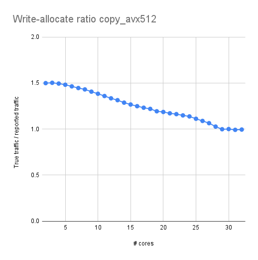
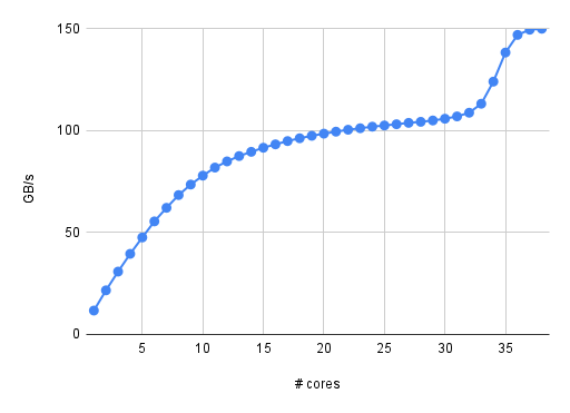
Himeno stencil benchmark: Roofline performance modeling and validation

[Update 17/11/29: Pointed out that the C version was modified from the original code – thanks Julian]

The Himeno benchmark [1] is a very popular code in the performance analysis and optimization community. Countless papers have been written that use it for performance assessment, prediction, optimization, comparisons, etc. Surprisingly, there is hardly a solid analysis of its data transfer properties. It’s a stencil code after all, and most of those can be easily analyzed.

The code

The OpenMP-parallel C version looks as shown below. I have made a slight change to the original code: The order of indices on the arrays a, b, and c hinders efficient SIMD vectorization, so I moved the short index to the first position. This also makes it equivalent to the Fortran version.

// all data structures hold single-precision values
for(n=0;n<nn;++n){
  gosa = 0.0;
  #pragma omp parallel for reduction(+:gosa) private(s0,ss,j,k)
  for(i=1 ; i<imax-1 ; ++i)
    for(j=1 ; j<jmax-1 ; ++j)
      for(k=1 ; k<kmax-1 ; ++k){
        // short index on a, b, c was moved up front
        s0 = a[0][i][j][k] * p[i+1][j ][k ]
           + a[1][i][j][k] * p[i ][j+1][k ]
           + a[2][i][j][k] * p[i ][j ][k+1]
           + b[0][i][j][k] * ( p[i+1][j+1][k ] - p[i+1][j-1][k ]
                             - p[i-1][j+1][k ] + p[i-1][j-1][k ] )
           + b[1][i][j][k] * ( p[i ][j+1][k+1] - p[i ][j-1][k+1]
                             - p[i ][j+1][k-1] + p[i ][j-1][k-1] )
           + b[2][i][j][k] * ( p[i+1][j ][k+1] - p[i-1][j ][k+1]
                             - p[i+1][j ][k-1] + p[i-1][j ][k-1] )
           + c[0][i][j][k] * p[i-1][j ][k ]
           + c[1][i][j][k] * p[i ][j-1][k ]
           + c[2][i][j][k] * p[i ][j ][k-1]
           + wrk1[i][j][k];
        ss = ( s0 * a[3][i][j][k] - p[i][j][k] ) * bnd[i][j][k];
        gosa = gosa + ss*ss;
        wrk2[i][j][k] = p[i][j][k] + omega * ss;
      }
  // copy-back loop ignored for analysis
  #pragma omp parallel for private(j,k)
  for(i=1 ; i<imax-1 ; ++i)
    for(j=1 ; j<jmax-1 ; ++j)
      for(k=1 ; k<kmax-1 ; ++k)
        p[i][j][k] = wrk2[i][j][k];
} /* end n loop */

Himeno stancil

Figure 1: Structure of the 19-point stencil showing the data access pattern to the p[][][] array in the Himeno benchmark. The k index is the inner (fast) loop index here.

There is an outer iteration loop over n. The first (parallel) loop nest over i, j, and k updates the wrk2 array from the arrays a, b, c, wrk1, bnd, and p, of which only p has a stencil-like access pattern (see Fig. 1). All others are accessed in a consecutive, cacheline-friendly way. Since the coefficient arrays a, b, and c carry a fourth index in the first position, the row-major data layout of the C language leads to many concurrent data streams. We will see whether or not this impacts the performance of the code.

A second parallel loop nest copies the result in wrk2 back to the stencil array p. This second loop can be easily optimized away (how?), so we ignore it in the following; all analysis and performance numbers pertain to the first loop only.

Amount of work

There are 14 floating-point additions, 7 subtractions, and 13 multiplications in the loop body. Hence, one lattice site update (LUP) amounts to 34 flops.

Data transfers and best-case code balance

For this analysis the working set shall be larger than any cache. It is straightforward to calculate a lower limit for the data transfers if we assume perfect spatial and temporal locality for all data accesses within one update sweep: All arrays except wrk2 must be read at least once, and wrk2 must be written. This leads to (13+1) single-precision floating-point numbers being transferred between the core(s) and main memory. The best-case code balance is thus Bc = 1.65 byte/flop = 56 byte/LUP. If the architecture has a write-back cache, an additional write-allocate transfer must be accounted for if it cannot be avoided (e.g., by nontemporal stores). In this case the best-case code balance is Bc = 1.76 byte/flop = 60 byte/LUP.

Considering that even the most balanced machines available today are not able to feed such a hunger for data (e.g., the new NEC-SX Aurora TSUBASA vector engine with 0.5 byte/flop), we know that this code will be memory bound. If the memory bandwidth can be saturated, the upper performance limit is the memory bandwidth divided by the code balance.

Continue reading