Georg Hager's Blog

Random thoughts on High Performance Computing

Content

A riddle in D/A conversion – and its solution

This post is not about high performance computing, for a change; it does, however, have a distinct performance-related vibe, so I think it qualifies for this blog. Besides, I had so much fun solving this riddle that I just cannot keep it to myself, so here goes.

D/A conversion with Arduino and ZN426

I was always interested in digital signal processing, and recently I decided to look into an old drawer and found a couple of ZN426E8 8-bit D/A converters that I had bought in the 80s. I asked myself whether a standard Arduino Uno with its measly 16 MHz ATmega 328 processor would be able to muster enough performance to produce waveforms in the audio range (up to at least a couple of kHz) by copying bytes from a pre-computed array to the D/A converter. The ZN426 itself wouldn’t be a bottleneck in this because it’s just an R-2R ladder with a worst-case settling time of 2 µs, which leads to a Nyquist frequency of 250 kHz. Ample headroom for audio. At 16 MHz, 2 µs means 32 clock cycles, so it shouldn’t really be a problem for the Arduino as well even with compiled code. Or so I thought.

ZN426E8

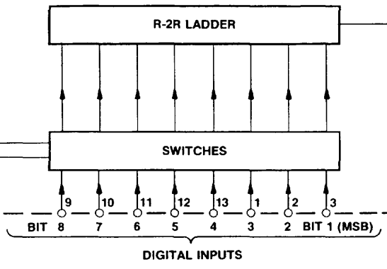
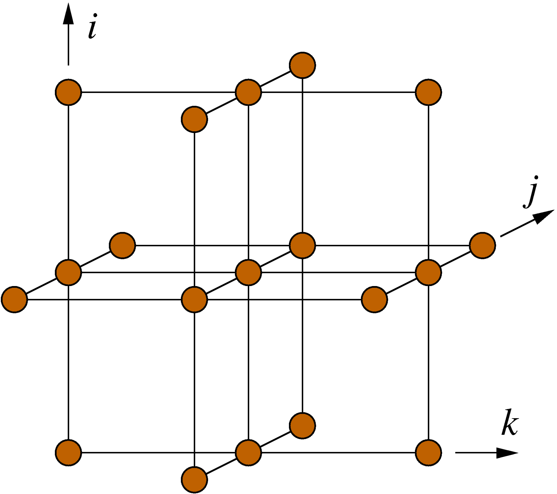
Fig. 1: The input lines of the D/A converter are numbered with bit 8 being the LSB (image cut from the Plessey data sheet for the ZN426E8)

So I hooked up the digital output lines of port D on the Uno to the input lines of the D/A converter and added the other necessary components according to the minimal example in the data sheet (basically a resistor and a capacitor needed by the internal 2.55 V reference). Unfortunately, the ZN426 data sheet uses an unusual numbering of the bits: bit 1 is the MSB, and bit 8 is the LSB. I missed that and inadvertently mirrored the bits, which led to an “interesting” waveform the first time I fired up the program. Now instead of fixing the circuit, I thought I could do that in software; just mirror the bits before writing them out to PORTD:

// output bytes in out[]
for(int i=0; i<N; i++) {
  unsigned char d=0;
  // mirror the bits in out[i], result in d
  for(int j=0; j<=7; ++j){
    unsigned char lmask = 1 << j, rmask = 128 >> j;
    if(out[i] & lmask) d |= rmask;
  }
  PORTD = out[i];
}

I knew that this was just a quick hack and that one could do it faster, but I just wanted the waveform to look right, and then care for performance. By the way, shift and mask operations should be fast, right? As a first test I wanted to approximate a square wave using Fourier synthesis:

f(t)=\sin t +\frac{1}{3}\sin 3t+\frac{1}{5}\sin 5t+\ldots
Fourier-synthesized square wave (first 20 harmonics) with wrong duty cylcle

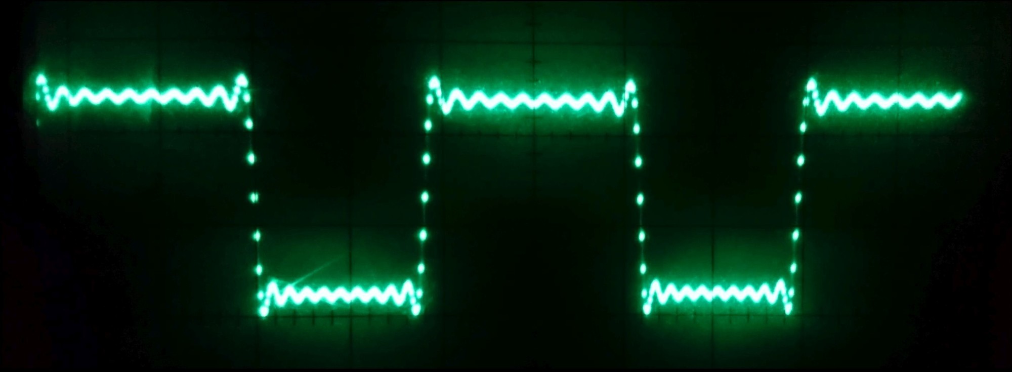
Fig. 2: Fourier-synthesized square wave (first 20 harmonics) with wrong duty cycle

The problem

Of course, the resulting function was then shifted and scaled appropriately to map to the range {0,…,255} of the D/A input. As a test, I used 200 data points per period and stopped at 20 harmonics (10 of which were nonzero). On first sight, the resulting waveform looked OK on the scope (see Fig. 2): the usual Gibbs phenomenon near the discontinuities, the correct number of oscillations. However, the duty cycle was not the expected 1:1 but more like 1.3:1. I first assumed some odd programming error, so I simplified the problem by using a single Fourier component, a simple sine wave. Figure 3 shows the result: It was obviously not a correct sine function, since the “arc” at the top is clearly blunter than that at the bottom. So it wasn’t some bug in the Fourier synthesis but already present in the fundamental harmonic.

This sine function is not quite a sine function

Fig. 3: This sine function is not quite a sine function

Bug hunting

In order to track the bug I made some experiments. First I compiled an adapted version of the code on my PC so I could easily inspect and plot the data in the program. It turned out that the math was correct – when plotting the out[] array, I got exactly what was expected, without distortions. Although this was reassuring, it left basically two options: Either it was an “analog” problem, i.e., something was wrong with the linearity of the D/A converter or with its voltage reference, or the timing was somehow off so that data points with high voltages took longer to output.

To check the voltage reference, I tried to spot fluctuations with the scope hooked up to it, but there was nothing – the voltage was at a solid 2.5 V (ish), and there was no discernible AC component visible within the limitations of my scope (a Hameg HM 208, by the way); a noise component of 20 mVpp would have been easily in range. The next test involved the timing: I inserted a significant delay (about 200 µs) after writing the byte to PORTD. This reduced the output frequency quite a bit since the original code spat out one byte about every 20 µs. Lo and behold – the asymmetries were gone. At this point it should have dawned on me, but I still thought it was an analog problem, somehow connected to the speed at which the D/A converter settles to the correct output voltage. However, the specs say that this should take at most 2 µs, so with one new value every 20 µs I should have been fine.

Correct duty cycle after rewiring the D/A input lines

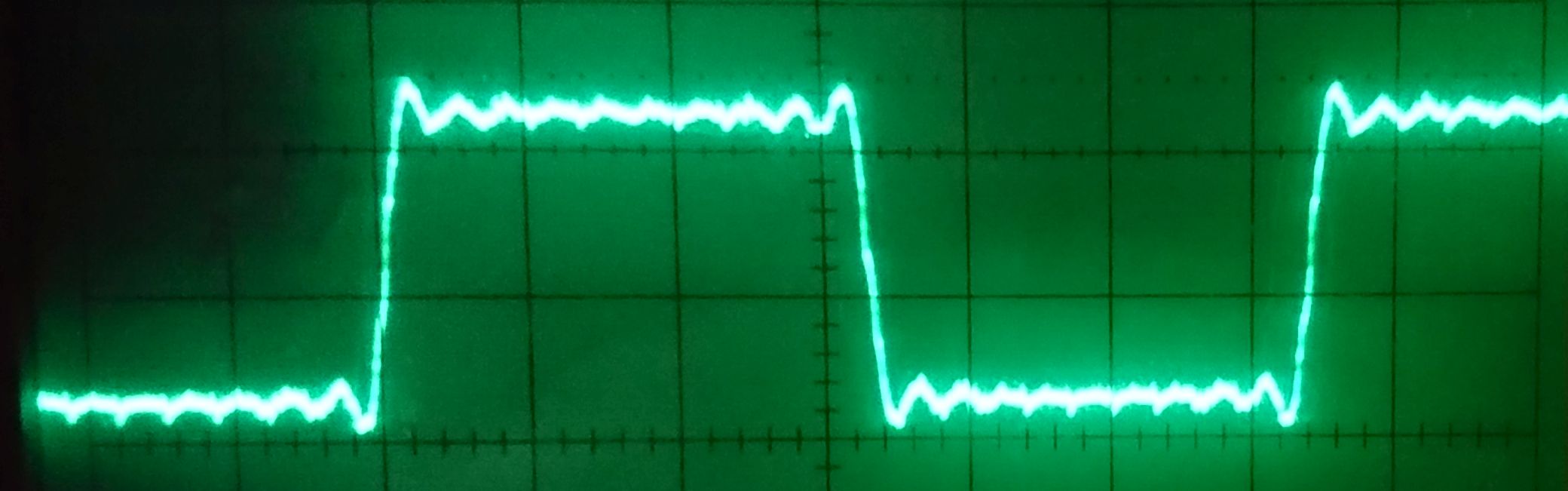
Fig. 4: Correct duty cycle after rewiring the D/A input lines

The solution

In the end, out of sheer desperation I decided to take out the last bit of complexity and rewired the D/A input bits so that the byte-mirror code became obsolete. Figure 4 shows the resulting output voltage for the square wave experiment. There are two major observations here: (1) The duty cycle was now correct at 1:1, and (2) the performance of the code was greatly improved. Instead of one value every 20 µs it now wrote one value every 550 ns (about 9 clock cycles). Problem solved – but why?

The observation that the nonlinearity disappeared when I inserted a delay was the key. In the byte-mirror code above, the more bits in the input byte out[i] are set to one, the more often the if() condition is true and the or-masking of the output byte d takes place. In other words, the larger the number of one-bits, the longer it takes to put together the output byte. And since voltages near the maximum are generated by numbers close to 255 (i.e., with lots of set bits), a phase in the output waveform with a large average voltage used a longer time step than one with a low average voltage. In other words, the time step had a component that was linear in the Hamming weight (or popcount) of the binary output value.

Of course I did some checks to confirm this hypothesis. Rewriting the byte-mirror code without an if condition (instead of rewiring the data lines) fixed the problem as well:

for(int i=0; i<N; i++) {
  unsigned char d=0,lmask=1,rmask=128,v;
  for(unsigned char j=0; j<=7; ++j){
    v = out[i] & lmask;
    d |= (v<<(7-j))>>j;
  }
  PORTD = d;
}

There are many ways to do this, but all resulted in (1) correct output and (2) slow code, more than an order of magnitude slower than the “plain” code with correctly wired data lines. Whatever I tried to mirror the bits, it always took a couple hundred cycles.

In summary, a problem which looked like a nonlinearity in a D/A converter output was actually caused by my code taking longer when more bits were set in the output, resulting in a larger time step for higher voltages.

Odds and ends

At a time step of roughly half a microsecond, the behavior of the D/A converter and the Arduino become visible

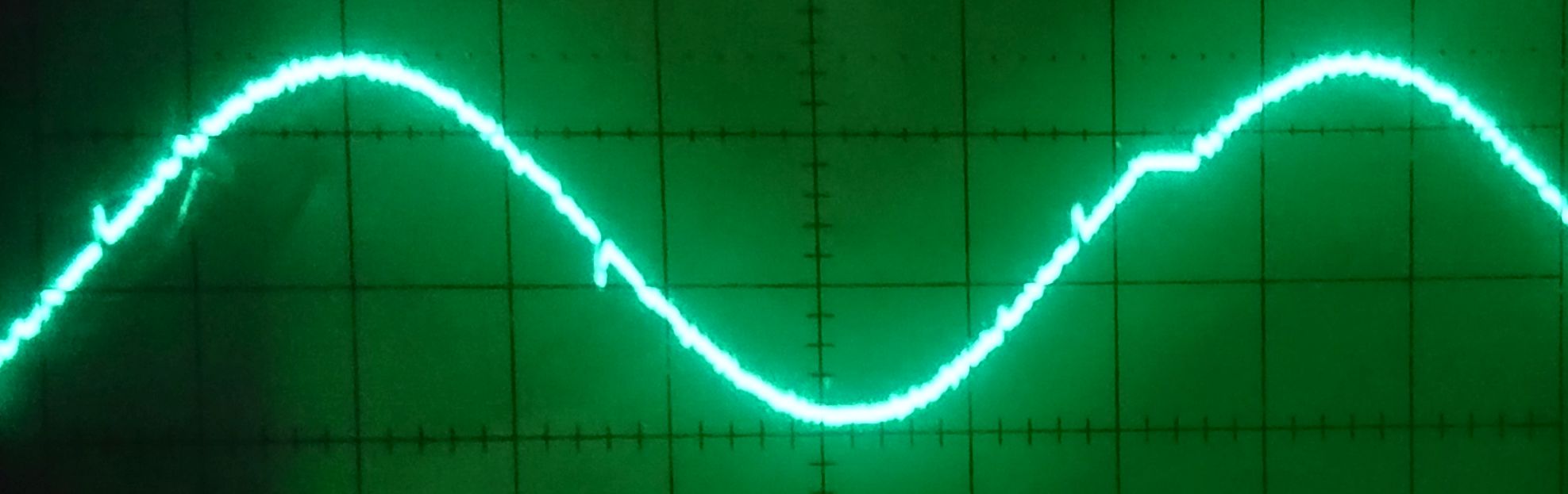
Fig. 5: At a time step of roughly half a microsecond, the behavior of the D/A converter and the Arduino become visible

Without mirroring, the time step between successive updates is much smaller than the worst-case settling time of the D/A converter. Figure 5 shows a pure sine function again. One can clearly discern spikes at the points where lots of input bits change concurrently, e.g., at half of the maximum voltage. I don’t know if this is caused by the outputs of the Arduino port being not perfectly synchronous, or if it is an inherent property of the converter. In practice it probably should not matter since there will be some kind of buffer/amplifier/offset compensation circuit that acts as a low-pass filter.

Figure 5 shows yet another oddity: From time to time, the Arduino seems to take a break (there is a plateau at about 75% of the width). This first showed up on the scope as a “ghost image,” i.e., there was a second, shifted version of the waveform on the screen. Fortunately, my Hameg scope has a builtin digital storage option, and after a couple of tries I could capture what is seen in Fig. 5. These plateaus are roughly 6-7 µs in length and turn up regularly every 1.1 ms or so. I checked that this is not something that occurs in between calls to the loop() function; it is really regular, and asynchronous to whatever else happens on the Arduino. I don’t know exactly what it is, but the frequency of these plateaus is suspiciously close to the frequency of the PWM outputs on pins 5 and 6 of the Uno (960 Hz), so it might have something to do with that.

You can download the code of the sketch here: dftsynth.c Remember that this is just a little test code. It only implements  a pure sine transform. I am aware that the Arduino Uno with its limited RAM is not the ideal platform for actually producing audio output.

Please drop me a note if you have any comments or questions.

EoCoE webinar on A64FX

Our friends from the “EoCoE-II” project have invited us to share our results about the new A64FX processor. Attendance is free and open to everyone. Please register using the link given below.


Title: The A64FX processor: Understanding streaming kernels and sparse matrix-vector multiplication

Date: November 18, 2020, 10:00 a.m. CET

Speakers: Christie L. Alappat and Georg Hager (RRZE)

Registration URL: https://attendee.gotowebinar.com/register/3926945771611115789

Abstract:  The A64FX CPU powers the current #1 supercomputer on the Top500 list. Although it is a traditional cache-based multicore processor, its peak performance and memory bandwidth rival accelerator devices. Generating efficient code for such a new architecture requires a good understanding of its performance features. Using these features, the Erlangen Regional Computing Center (RRZE) team will detail how they construct the Execution-Cache-Memory (ECM) performance model for the A64FX processor in the FX700 supercomputer and validate it using streaming loops. They will describe how the machine model points to peculiarities in the microarchitecture to keep in mind when optimizing applications, and how, applying the ECM model to sparse matrix-vector multiplication (SpMV), they motivate why the CRS matrix storage format is inappropriate and how the SELL-C-sigma format can achieve bandwidth saturation for SpMV. In this context, they will also look into some code optimization strategies that are relevant for A64FX and compare SpMV performance with AMD Rome, Intel Cascade Lake and NVIDIA V100.

This webinar is organized by the European Energy-Oriented Center of Excellence (EoCoE). A video recording is now available on the EoCoE YouTube channel:

Intel’s port 7 AGU blunder

Everyone’s got their pet peeves: For Poempelfox it’s Schiphol Airport, for Andreas Stiller it’s the infamous A20 gate. Compared to those glorious fails, my favorite tech blunder is a rather measly one, and it may not be relevant to many users in practice. However, it’s not so much the importance of it but the total mystery of how it came to happen. So here’s the thing.

Loads, stores, and AGUs

Sandy Bridge and Ivy Bridge LOAD and STORE units, AGUs, and their respective ports.

The Intel Sandy Bridge and Ivy Bridge architectures have six execution ports, two of which (#2 & #3) feed one LOAD pipeline each and one (#4) feeds a STORE pipe. These units are capable of transferring 16 bytes of data per cycle each. With AVX code, the core is thus able to sustain one full-width 32-byte LOAD (in two adjacent 16-byte chunks) and one half of a 32-byte STORE per cycle. But the LOAD and STORE ports are not the only thing that’s needed to execute these instructions – the core must also generate the corresponding memory addresses, which can be rather complicated. In a LOAD instruction like:

vmovupd ymm0, [rdx+rsi*8+32]

the memory address calculation involves two integer add operations and a shift. It is the task of the address generation units (AGUs) to do this. Each of ports 2 and 3 serves an AGU in addition to the LOAD unit, so the core can generate two addresses per cycle – more than enough to sustain the maximum LOAD and STORE throughput with AVX.

The peculiar configuration of LOAD and STORE units and AGUs causes some strange effects. For instance, if we execute the Schönauer vector triad: Continue reading

Node-Level Performance Engineering Course at LRZ

We proudly present a retake of our PRACE course on “Node-Level Performance Engineering” on December 3-4, 2019 at LRZ Garching.

This course covers performance engineering approaches on the compute node level. Even application developers who are fluent in OpenMP and MPI often lack a good grasp of how much performance could at best be achieved by their code. This is because parallelism takes us only half the way to good performance. Even worse, slow serial code tends to scale very well, hiding the fact that resources are wasted. This course conveys the required knowledge to develop a thorough understanding of the interactions between software and hardware. This process must start at the core, socket, and node level, where the code gets executed that does the actual computational work. We introduce the basic architectural features and bottlenecks of modern processors and compute nodes. Pipelining, SIMD, superscalarity, caches, memory interfaces, ccNUMA, etc., are covered. A cornerstone of node-level performance analysis is the Roofline model, which is introduced in due detail and applied to various examples from computational science. We also show how simple software tools can be used to acquire knowledge about the system, run code in a reproducible way, and validate hypotheses about resource consumption. Finally, once the architectural requirements of a code are understood and correlated with performance measurements, the potential benefit of code changes can often be predicted, replacing hope-for-the-best optimizations by a scientific process.

This is a two-day course with demos. It is provided free of charge to members of European research institutions and universities.

 Date: Tuesday, Dec 3, 2019 09:00 – 17:00
Wednesday, Dec 4, 2019 09:00 – 17:00
Location: LRZ Building, University campus Garching, near Munich, Hörsaal H.E.009 (Lecture hall)
Course webpage with detailed agenda: https://events.prace-ri.eu/event/901/
Registration: Via https://events.prace-ri.eu/event/901/registrations/633/

PPAM 2019 Workshops Best Paper Award for Dominik Ernst

Best Paper Award PPAM 2019

Dominik and his PPAM Best Poster Award

Our paper “Performance Engineering for a Tall & Skinny Matrix Multiplication Kernel on GPUs” by Dominik Ernst, Georg Hager, Jonas Thies, and Gerhard Wellein just received the best workshop paper award at the PPAM 2019, the 13th International Conference on Parallel Processing and Applied Mathematics, in Bialystok, Poland. In this paper, Dominik investigated different methods to optimize an important but often neglected computational kernel: the multiplication of two extremely non-square matrices, with millions of rows but very few (tens of) columns. Vendor libraries still do not perform well in this situation, so you have to roll your own implementation, which is a daunting task because of the huge optimization parameter space, especially on GPGPUs.

The optimizations were guided by the Roofline model (hence “Performance Engineering”), which provides an upper limit for the performance of the kernel. On an Nvidia V100 GPGPU, Dominik’s solution achieves more than 90% of the maximum performance for matrices with up to 40 columns, and more than 50% at up to 64 columns. This is significantly faster than vendor libraries at the time of writing.

The work was funded by the project ESSEX (Equipping Sparse Solvers for Exascale) within the DFG priority programme 1648 (SPPEXA). A preprint of the paper is available at arXiv:1905.03136.

Himeno stencil benchmark: ECM model, SIMD, data layout

In a previous post I have shown how to construct and validate a Roofline performance model for the Himeno benchmark. The relevant findings were:

  • The Himeno benchmark is a rather standard stencil code that is amenable to the well-known layer condition analysis. For in-memory data sets it achieves a performance that is well described by the Roofline model.
  • The performance potential of spatial blocking is limited to about 10% in the saturated case (on a Haswell-EP socket), because the data transfers are dominated by coefficient arrays with no temporal reuse.
  • The large number of concurrent data streams through the cache hierarchy and into memory does not hurt the performance, at least not too much. We had chosen a version of the code which was easy to vectorize but had a lot of parallel data streams (at least 15, probably more if layer conditions are broken).

Some further questions pop up if you want more insight: Is SIMD vectorization relevant at all? Does the data layout matter? What is the single-core performance in relation to the saturated performance, and why? All these questions can be answered by a detailed ECM model, and this is what we are going to do here. This is a long post, so I provide some links to the sections below:

Continue reading

Himeno stencil benchmark: Roofline performance modeling and validation

[Update 17/11/29: Pointed out that the C version was modified from the original code – thanks Julian]

The Himeno benchmark [1] is a very popular code in the performance analysis and optimization community. Countless papers have been written that use it for performance assessment, prediction, optimization, comparisons, etc. Surprisingly, there is hardly a solid analysis of its data transfer properties. It’s a stencil code after all, and most of those can be easily analyzed.

The code

The OpenMP-parallel C version looks as shown below. I have made a slight change to the original code: The order of indices on the arrays a, b, and c hinders efficient SIMD vectorization, so I moved the short index to the first position. This also makes it equivalent to the Fortran version.

// all data structures hold single-precision values
for(n=0;n<nn;++n){
  gosa = 0.0;
  #pragma omp parallel for reduction(+:gosa) private(s0,ss,j,k)
  for(i=1 ; i<imax-1 ; ++i)
    for(j=1 ; j<jmax-1 ; ++j)
      for(k=1 ; k<kmax-1 ; ++k){
        // short index on a, b, c was moved up front
        s0 = a[0][i][j][k] * p[i+1][j ][k ]
           + a[1][i][j][k] * p[i ][j+1][k ]
           + a[2][i][j][k] * p[i ][j ][k+1]
           + b[0][i][j][k] * ( p[i+1][j+1][k ] - p[i+1][j-1][k ]
                             - p[i-1][j+1][k ] + p[i-1][j-1][k ] )
           + b[1][i][j][k] * ( p[i ][j+1][k+1] - p[i ][j-1][k+1]
                             - p[i ][j+1][k-1] + p[i ][j-1][k-1] )
           + b[2][i][j][k] * ( p[i+1][j ][k+1] - p[i-1][j ][k+1]
                             - p[i+1][j ][k-1] + p[i-1][j ][k-1] )
           + c[0][i][j][k] * p[i-1][j ][k ]
           + c[1][i][j][k] * p[i ][j-1][k ]
           + c[2][i][j][k] * p[i ][j ][k-1]
           + wrk1[i][j][k];
        ss = ( s0 * a[3][i][j][k] - p[i][j][k] ) * bnd[i][j][k];
        gosa = gosa + ss*ss;
        wrk2[i][j][k] = p[i][j][k] + omega * ss;
      }
  // copy-back loop ignored for analysis
  #pragma omp parallel for private(j,k)
  for(i=1 ; i<imax-1 ; ++i)
    for(j=1 ; j<jmax-1 ; ++j)
      for(k=1 ; k<kmax-1 ; ++k)
        p[i][j][k] = wrk2[i][j][k];
} /* end n loop */

Himeno stancil

Figure 1: Structure of the 19-point stencil showing the data access pattern to the p[][][] array in the Himeno benchmark. The k index is the inner (fast) loop index here.

There is an outer iteration loop over n. The first (parallel) loop nest over i, j, and k updates the wrk2 array from the arrays a, b, c, wrk1, bnd, and p, of which only p has a stencil-like access pattern (see Fig. 1). All others are accessed in a consecutive, cacheline-friendly way. Since the coefficient arrays a, b, and c carry a fourth index in the first position, the row-major data layout of the C language leads to many concurrent data streams. We will see whether or not this impacts the performance of the code.

A second parallel loop nest copies the result in wrk2 back to the stencil array p. This second loop can be easily optimized away (how?), so we ignore it in the following; all analysis and performance numbers pertain to the first loop only.

Amount of work

There are 14 floating-point additions, 7 subtractions, and 13 multiplications in the loop body. Hence, one lattice site update (LUP) amounts to 34 flops.

Data transfers and best-case code balance

For this analysis the working set shall be larger than any cache. It is straightforward to calculate a lower limit for the data transfers if we assume perfect spatial and temporal locality for all data accesses within one update sweep: All arrays except wrk2 must be read at least once, and wrk2 must be written. This leads to (13+1) single-precision floating-point numbers being transferred between the core(s) and main memory. The best-case code balance is thus Bc = 1.65 byte/flop = 56 byte/LUP. If the architecture has a write-back cache, an additional write-allocate transfer must be accounted for if it cannot be avoided (e.g., by nontemporal stores). In this case the best-case code balance is Bc = 1.76 byte/flop = 60 byte/LUP.

Considering that even the most balanced machines available today are not able to feed such a hunger for data (e.g., the new NEC-SX Aurora TSUBASA vector engine with 0.5 byte/flop), we know that this code will be memory bound. If the memory bandwidth can be saturated, the upper performance limit is the memory bandwidth divided by the code balance.

Continue reading

Preview for SC15 tutorial on “Node-Level Performance Engineering” now available

SC15 solicits video previews of accepted tutorials for the first time this year. So watch the commercial for our SC15 full-day tutorial “Node-Level Performance Engineering“!

Kudos to Jörn Rüggeberg from the RRZE multimedia center for putting together this great piece of art.

Fooling the masses – Stunt 10: Always emphasize the “interesting” part of your work!

(See the prelude for some general information on what this is all about)

Have you ever thought about how to improve the aerodynamic properties of bulldozers? Yes? Then this stunt is for you.

Bulldozer aeodynamics

Figure 1: Always focus on the interesting stuff!

Code optimization is quite rewarding at times. You put all your effort into mutilating a chunk of code beyond all recognition, and in the end you get a 50% speedup. Often enough, this work requires a great deal of  expertise at the interface between hardware and software. And you certainly want to present your success to your peers so they understand how advanced you are.

If you do such a thing, don’t bother picking the low-hanging fruits. When 95% of the run time goes into a boring loop nest which multiplies a dense matrix with a vector, there is not much you can do beyond the standard textbook stuff – or use a library altogether. However, if the remaining 5% consist of a convoluted communication scheme, you’ve found your target. The fact that the possible gain is at most 5% shouldn’t stop you, because it’s all a matter of presentation; see Fig. 1: 3D bars and a proper choice of scales on the axes guide the reader’s eye and help you drive home your point. It’s like presenting the optimized drag coefficient of your aerodynamically improved bulldozer on high gloss paper, and the boring technical data in small black print on a dark blue background, on the back page.

Interestingly, if the optimization target is communication, or synchronization, or any other non-computational overhead, this stunt can be made to work even better: When you strongly scale to a pointless number of workers, reducing such overheads will give you arbitrary speedups, far beyond the factor of two that is theoretically possible if you restrict yourself to a sensible minimum parallel efficiency of 50%. Coming back to the heavy gear analogy, if you accelerate your bulldozer to 200 mph, the drag coefficient does become essential, and you may feel vindicated. It won’t solve any real-world problem, but hey, this is research after all.

Thanks to Gerhard Wellein for discovering this stunt in a paper. Many papers, actually.

A case for the non-temporal store

Non-temporal stores (also called “streaming stores”) were added to x86 processors with SSE2 (i.e. when the first Pentium IV called “Willamette” appeared in 2000). There was also some support in MMX before, but nobody should be required to use MMX any more. In contrast to standard store instructions which transfer data from registers to memory, NT stores do not require a prior cache line read for ownership (RFO) but write to memory “directly” (well not quite – but to first order it’s true). Beware the usual explanations for RFO that Google finds for you – they almost all describe RFO as something inherently connected to cache coherency in multi-processor systems, but RFO is also required on a single core, whenever there is a cache that is organized in lines.

What are NT stores good for? Again, most references cite them as a means to avoid cache pollution in cases where stored data will not be re-used soon. That’s true to some extent; every word that you don’t store in your cache means more room for other, more frequently used data. But that’s only one half the story. Imagine you have a code whose working set fits into the outer-level cache and which produces data to be stored in memory. Using NT stores for such a code will probably slow it down because, depending on the LD/ST balance, performance is then limited by the memory interface. The true benefit of NT stores can be seen with a truly memory-bound code which is not dominated by loads, like, e.g., the STREAM COPY benchmark, relaxation methods, the lattice-Boltzmann algorithm, or anything that can be formulated in terms of stride-one store streams: By saving the RFO, the pressure on the memory subsystem is reduced. See, e.g., my talk at the KONWIHR results and review workshop in December 2007 at LRZ where the performance boost through NT stores was demonstrated using a 2D Jacobi (5-point stencil) code.

The most important non-temporal store instruction is movntpd, which writes the contents of a full 16-byte SSE register (xmm0…xmm15) to memory. The memory address has to be a multiple of 16, else an exception will be generated. Also, this instruction exists in a “packed” variant only, i.e. there is no movntsd that would only store the lower 8 bytes of the register (AMD has included it, though, into their SSE4a extensions which are implemented with the K10 CPUs – read a nice writeup by Rahul Chaturvedi from AMD for more information). So, if you are stuck with Intel processors or a compiler which does not know about movntsd on K10, loops which use NT stores must be vectorizable and the store stream(s) must be 16-byte aligned.

Or so I thought, for a long time. This assumption was backed, of course, by stupid compilers who blatantly refused to use NT stores if they weren’t 100% sure at compile time whether the store stream was actually aligned. Never heard of loop peeling, eh? Thank goodness great Intel gave us the vector aligned pragma, which you can put in front of a loop in order to tell the compiler that the streams appearing inside the loop were 16-byte aligned! But that always refers to all streams, including reads, and if you somehow forget to pay proper attention, you’re immediately punished by an exception again. To make a long story short, you never really know what’s going on inside the compiler’s twisted little brain, and the diagnostics don’t help either (“LOOP WAS VECTORIZED”, yes, thank you very much).

In hope for some future improvement (unaligned NT store? Or *gasp* maybe even a scalar one?) I looked into Intel’s AVX extensions for SSE, to be implemented in the Sandy Bridge processor, which is to follow Westmere in 2010. That would be a “Streaming SIMD Extension Extension”, right? Whatever, there is neither a scalar nor an unaligned packed NT store in there. But I stumbled across something that had been there since SSE2: The beautiful maskmovdqu instruction. From the manual:


MASKMOVDQU xmm1,xmm2 – Store Selected Bytes of Double Quadword with NT Hint

Stores selected bytes from the source operand (first operand) into an 128-bit memory location. The mask operand (second operand) selects which bytes from the source operand are written to memory. The source and mask operands are XMM registers. The location of the first byte of the memory location is specified by DI/EDI/RDI and DS registers. The memory location does not need to be aligned on a natural boundary. […]


Way cool. Although the fixed address register is somewhat inflexible, the instruction is even better than pure scalar or pure unaligned NT store – it can store any part of an XMM register, down to the byte level, and with no alignment restrictions. And there’s a C/C++ compiler intrinsic, too. That has made it easy to implement our beloved vector triad in explicit SSE. These are two possible variants:

Scalar (unaligned) Packed unaligned
  __m128d xmm1,xmm2,xmm3,xmm4;
  __m128i mask_low=_mm_set_epi32(0,0,-1,-1);
#pragma omp parallel private(j)
{
if(size > 1000000) {
  for(j=0; j<niter; j++){
#pragma omp for private(xmm1,xmm2,xmm3,xmm4)
    for(i=0; i<size; i++) {
      xmm1 = _mm_load_sd(d+i);
      xmm2 = _mm_load_sd(c+i);
      xmm3 = _mm_load_sd(b+i);
      xmm4 = _mm_mul_sd(xmm1,xmm2);
      xmm4 = _mm_add_sd(xmm4,xmm3);
      _mm_maskmoveu_si128(reinterpret_cast<__m128i>(xmm4), mask_low, (char*)(a+i));
    }
  }
} else {
// same with standard store
}
  __m128d xmm1,xmm2,xmm3,xmm4;
  __m128i mask_all=_mm_set_epi32(-1,-1,-1,-1);
#pragma omp parallel private(j)
{
if(size > 1000000) {
  for(j=0; j<niter; j++){
#pragma omp for private(xmm1,xmm2,xmm3,xmm4,xmm5)
    for(i=0; i<size; i+=2) {
      xmm1 = _mm_load_pd(d+i);
      xmm2 = _mm_load_pd(c+i);
      xmm3 = _mm_load_pd(b+i);
      xmm4 = _mm_mul_pd(xmm1,xmm2);
      xmm4 = _mm_add_pd(xmm4,xmm3);
      _mm_maskmoveu_si128(reinterpret_cast<__m128i>(xmm4), mask_all, (char*)(a+i));
    }
  }
} else {
// same with standard store
}

The left one is an example for a purely scalar code which employs NT stores. The right one shows how a vectorized code can be endowed with NT stores if 16-byte alignment cannot be enforced. The compiler does neither by itself. Of course, NT stores only make sense if the arrays are large. I have set the lower limit to N=1000000, which is largish compared to the cache sizes but neatly shows the effect of NT vs. standard store:

The figure includes standard scalar versions without NT stores as well. Obviously, the maskmovdqu instruction does the job. There is hardly any performance loss in the serial case, and none at all with four threads. I have omitted any comment on in-cache behavior of the different variants; this is a separate story (and one which becomes more interesting once Nehalem is out!).

If you want to know more about using SSE intrinsics in C/C++ code, the Intel C++ Compiler for Linux Intrinsics Reference is for you.