(See the prelude for some general information on what this is all about)
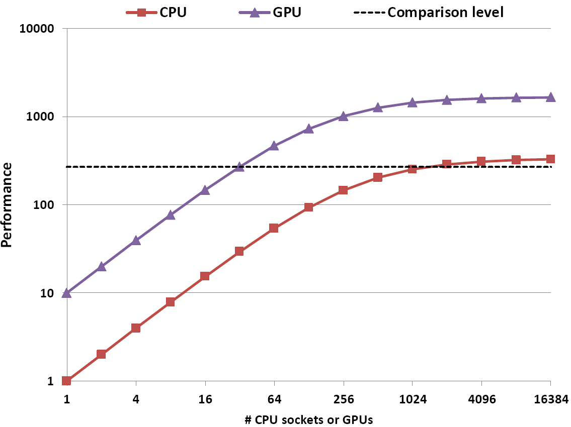
Fig. 1: Comparing performance vs. number of compute units (CPU sockets, GPUs) under limited scalability can yield any result if you do it right!
Strong scaling performance comparisons between standard (i.e., CPU-based) and accelerated (e.g., GPU-based) systems are particularly rewarding, since there is ample opportunity to generate any speedup number you want. It is not about fabricating a large GPU vs. CPU speedup – this special topic deserves its own stunt (stay tuned!). You can just as well apply it to a “baseline” vs. an “optimized” code on the same machine.
This may not be easy to digest on a theoretical level, so I explain it using an example: Assume we have a parallel CPU code whose strong scalability is limited by Amdahl’s Law with a serial runtime fraction of 0.3%. Hence, the speedup factor is limited to 333. A parallel GPGPU version of the same program achieves a speedup of 10 (compared to one CPU socket) for the parallel part, and of 5 for the sequential part. Figure 1 shows a performance comparison for up to 16384 compute units (CPU sockets or GPUs, respectively). As expected, the GPGPU speedup is 10 for small numbers of workers and goes down to 5 for large numbers – always comparing equal numbers of GPGPUs and CPU sockets. So far so good.
However, if you pose the right question, the factor can be much larger – even infinity, if you want: If we ask “How many CPU sockets do we need to outcompute 32 GPUs?”, the answer is clearly 2048. This means that your GPU-vs-CPU speedup is not 5, and also not 10, but almost 64 (see the dashed line in the graph). And its gets even better: Somewhere between 32 and 40 GPUs the required number of CPU sockets slips away to infinity! Your GPUs can go where no CPU has ever gone before (and never will)!
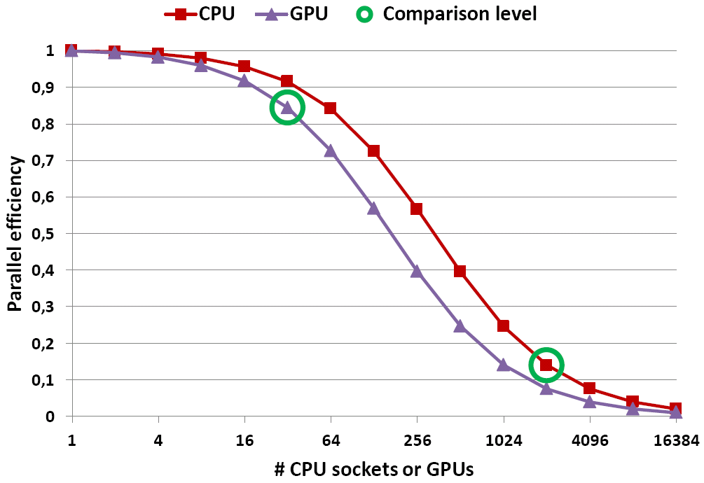
Fig. 2: Plotting the parallel efficiency of both variants reveals the reason why the stunt works. Note that the efficiency of the GPU version is always worse.
The reason why this works is that you compare the two graphs at different numbers of workers – so different that the parallel efficiency for the CPU code is way down, whereas for the GPU code it is still acceptable (see Fig. 2)! Or to put it the other way round: If we compare equal numbers of workers on both sides, the parallel efficiency on the CPUs is always better.
The sensible way to compare achievable performance would be to set a certain practical lower limit for the parallel efficiency, e.g., 50%. From a computing center point of view, this is probably the lowest efficiency we’d be willing to accept, except in cases where the reason for going parallel is lack of memory. Scaling beyond that point does not make sense, not even for the purpose of comparison! A reasonable question to ask would be “How much performance can I get from the two codes at their respective minimum acceptable efficiency point?”
So the gist of it is: When comparing scaled performance data, ask the right questions and be the hero of the day. And don’t talk about parallel efficiency, or people might ask why you are wasting precious CPU cycles…
Thanks to Gerhard for discovering this extraordinary stunt!