Georg Hager's Blog

Random thoughts on High Performance Computing

Content

Blaze 2.1 has been released

Blaze is an open-source, high-performance C++ math library for dense and sparse arithmetic based on Smart Expression Templates. Just in time for ISC’14, Blaze 2.1 has been released. The focus of this latest release is the improvement and extension of the shared memory parallelization capabilities: In addition to OpenMP parallelization, Blaze 2.1 now also enables shared memory parallelization based on C++11 and Boost threads.  Additionally, the underlying architecture for the parallel execution and automatic, context-sensitive optimization has been significantly improved. This not only improves the performance but also allows for an efficient parallel handling of computations involving block-structured vectors and matrices.

All of the Blaze documentation and code can be downloaded at https://code.google.com/p/blaze-lib/.

Bill Gropp on “Engineering for Performance in High Performance Computing”

At the PASC14 conference in Zurich, Bill Gropp gave a great talk on Performance Engineering, the way it should be done. 100% along the lines of what we try to teach people in our tutorials! https://www.youtube.com/watch?v=sadfSARXSC0

Gaussian Elimination Squad wins Intel Parallel Universe Computing Challenge at SC13!

PUCC-bracket

Final team bracket for the Intel Parallel Universe Computing Challenge

We’ve made it! The final round against the “Coding Illini” team, comprising members from the University of Illinois and the National Center for Supercomputing Applications (NCSA), took place on Thursday, November 21, at 2pm Mountain Time. We were almost 30% ahead of the other team after the trivia, and managed to extend that head start in the coding challenge, which required the parallelization of a histogram computation. This involved quite a lot of typing, since OpenMP does not allow private clauses and reductions for arrays in C++. My request for a standard-sized keyboard was denied so we had to cope with a compact one, which made fast typing a little hard. As you can see in the video, a large crowd had gathered around the Intel booth to cheer for their teams.

Remember, each match consisted of two parts: The first was a trivia challenge with 15 questions about computing, computer history, programming languages, and the SC conference series. We were given 30 seconds per question, and the faster we logged in the correct answer (out of four), the more points we got. The second part was a coding challenge, which gave each team ten minutes to speed up a piece of code they had never seen before as much as possible. On top of it all, the audience could watch what we were doing on two giant screens.

The Gaussian Elimination Squad

The Gaussian Elimination Squad: (left to right) Michael Kluge, Michael Ott, Joachim Protze, Christian Iwainsky, Christian Terboven, Guido Juckeland, Damian Alvarez, Gerhard Wellein, and Georg Hager (Image: S. Wienke, RWTH Aachen)

In the first match against the Chinese “Milky Way” team, the code was a 2D nine-point Jacobi solver; an easy task by all means. We did well on that, with the exception that we didn’t think of using non-temporal stores for the target array, something that Gerhard and I had described in detail the day before in our tutorial! Fortunately, the Chinese had the same problem and we came out first. In the semi-final against Korea, the code was a multi-phase lattice-Boltzmann solver written in Fortran 90. After a first surge of optimism (after all, LBM has been a research topic in Erlangen for more than a decade) we saw that the code was quite complex. We won, but we’re still not quite sure whether it was sheer luck (and the Korean team not knowing Fortran). Compared to that, the histogram code in the final match was almost trivial apart from the typing problem.

The back image on our shirts

According to an enthusiastic spectator we had “the nerdiest team name ever!”

After winning the challenge, the “Gaussian Elimination Squad” proudly presented a check for a $25,000 donation to the benefit of the Philippines Red Cross.

I think that all teams did a great job, especially when taking into account the extreme stress levels caused by the insane time limit, and everyone watching the (sometimes not-so-brilliant) code that we wrote! It’s striking that none of the US HPC leadership facilities made it to the final match – they all dropped out in the first round (see the team bracket above).

The Gaussian Elimination Squad represented the German HPC community, with members from RWTH Aachen (Christian Terboven and Joachim Protze), Jülich Supercomputing Center (Damian Alvarez), ZIH Dresden (Michael Kluge and Guido Juckeland), TU Darmstadt (Christian Iwainsky), Leibniz Supercomputing Center (Michael Ott), and Erlangen Regional Computing Center (Gerhard Wellein and Georg Hager). Only four team members were allowed per match, but the others could help by shouting advice and answers they thought were correct.


Gaussian Elimination Squad to fight in “SC13 Intel Parallel Universe Computing Challenge”

It seems that Intel’s marketing division has some money to spend for charity – $25,000 to be exact. To make its spending as entertaining as possible, they have set up a stage show at SC13 in Denver, Colorado (Nov 17-22, 2013): The “Intel Parallel Universe Computing Challenge.”

Eight teams from the US, Europe, China, and Korea are going to fight in a three-round sudden death tournament. The German team comprises members from Aachen, Darmstadt, Jülich, Dresden, Garching, and Erlangen, and happens to be led by me. According to the rules each match will be 30 minutes, in which the teams have to answer questions and optimize code. The audience will have the chance to answer questions and win prizes, too! So if you happen to be at SC13 and can spare the time, drop by the Intel booth (#2701, see floor plan) and see us fight! See the link above for the schedule.

Honoring one of the greatest mathematicians of all time, the German team has chosen a peculiar war name: The “Gaussian Elimination Squad.” We will take on “Team Milky Way” from China in our first match on Tuesday, Nov 19th, 11:00am. We do not know why they have picked the name of a popular chocolate bar 😉 but probably it was in anticipation of what’s going to happen to them:

Milky Way before processing

Milky Way before elimination

Milky Way after processing

Milky Way after elimination


Now you know why we call ourselves the “Gaussian Elimination Squad.”

Intel vs. GCC for the OpenMP vector triad: Barrier shootout!

We use the Schönauer Vector Triad for most of our microbenchmarking. It’s a simple benchmark that everyone can write. It looks quite simple when parallelized with OpenMP:

double precision, dimension(N) :: a,b,c,d
! initialization etc. omitted
s = walltime()
!$omp parallel private(R,i)
do R=1,NITER
!$omp do
  do i=1,N
    a(i) = b(i) + c(i) * d(i)
  enddo
!$omp end do
enddo
!$omp end parallel
e=walltime()
MFlops = R*N/(e-s)/1.e6

There are some details that are necessary to make it work as intended; you can read all about this in our book [1]. Usually we choose NITER for every N so that the runtime is a couple hundred milliseconds (so it can be measured accurately), and report performance for N ranging from small to large. The performance of the vector triad is determined by the data transfers, even when the data is in the L1 cache. In the parallel case we can additionally see the usual multicore bandwidth bottleneck(s).

The OpenMP parallelization adds its own overhead, of course. As it turns out, it is mostly concentrated in the implicit barrier at the end of the workshared loop in this case. So, when looking at the performance of the OpenMP code vs. N, we usually see that using more threads slows down the code if N is too small. We can even calculate the barrier overhead from this (again, the book will tell you the gory details).

The barrier overhead varies across compilers and compiler versions, and it depends on the positions of the threads in the machine (e.g., sharing caches or not). You can certainly measure it directly with a suitable microbenchmark [2], but it is quite interesting to see the impact directly in the vector triad performance data.

vtriad_Lima_icpc_vs_gcc

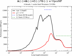
Here we see the OpenMP vector triad performance on one “Intel Xeon Westmere” socket (6 cores) running at about 2.8 GHz, comparing a reasonably current Intel compiler with g++ 4.7.0. With the Intel compiler the sequential code achieves “best possible” performance within the L1 cache (4 flops in 3 cycles). With OpenMP turned on you cannot see this, of course, since the barrier overhead dominates for loop lengths below a couple of 1000s.

Looking at the results for the two compilers we see that GCC has not learned anything over the last five years (this is for how long we have been comparing compilers in terms of OpenMP barrier overhead): The barrier takes roughly a factor of 20 longer with gcc than with the Intel compiler. Comparing with the ECM performance model [3] for the vector triad we see that the Intel compiler’s barrier is fast enough to at least get near the performance limit in the L2 cache (blue dashed line). Both compilers are on par where it’s easy, i.e., in L3 cache and memory, where the loop is so long that the overhead is negligible.

Note that the bad performance of g++ in this benchmark is not due to some “magic” compiler option that I’ve missed. It’s the devastatingly slow OpenMP barrier. For reference, these are the compiler options I have used:

icpc -openmp -Ofast -xHOST -fno-alias ...
g++ -fopenmp -O3 -msse4.2 -fargument-noalias-global ...

In conclusion, the GCC OpenMP barrier is still slooooow. If you have “short” loops to parallelize, GCC is not for you. Of course you might be able to work around such problems (mutilating a popular saying from one of the Great Old Ones: “If synchronization is the problem, don’t synchronize!”), but it’s still good to be aware of them.

If you are interested in concrete numbers you can take a look at any of our recent tutorials [4], where we always include some recent barrier measurements with current compilers.

[1] G. Hager and G. Wellein: Introduction to High Performance Computing for Scientists and Engineers. CRC Press, 2010.

[2] The EPCC OpenMP Microbenchmarks.

[3] G. Hager, J. Treibig, J. Habich, and G. Wellein: Exploring performance and power properties of modern multicore chips via simple machine models. Computation and Concurrency: Practice and Experience, DOI: 10.1002/cpe.3180 (2013), Preprint: arXiv:1208.2908

[4] My Tutorials blog page

The 400x GPU speedup baloney

Recently, in the HPC services office…

(… phone rings …)

“Computing Center, HPC services. How can I help you?”

“Yes, High Performance Computing.”

“You want to use our GPGPU cluster? Great! The load on this baby could be higher anyway. It’s hard to believe, but people seem to avoid it like the plague (jovial laughter). Do you have a code that runs on GPUs already?”

“I see, the compiler should be able to handle this. But the code is SIMD vectorized for standard processors, right?”

“No, this has nothing to do with cell phones. SIMD means ‘Single Instruction Multiple Data,’ i.e., several operations can be performed on different operands with a single machine instruction. If that works, chances are that the program can be run efficiently on a GPU as well. After all, GPUs implement the SIMD principle quite extensively.”

“Hm? I think I don’t understand…”

“Ah, ok. No, you don’t have to learn assembly programming to do this. But you may have to think a little more about how the compiler looks at your code. Often you can help it by supplying additional information, like source directives. And of course you need to use a compiler that understands what SIMD is. Alas, the GNU compilers don’t have a clue about it, mostly. By the way, how  have you parallelized the code?”

“Um, no. Compilers can’t help you much here, except for very simple cases where a 10-year-old can do it just as well. But you do have to parallelize. How do you want to draw a meaningful comparison to the GPU version?”

“What do you mean, you don’t need to do this?”

“Um, yes, I think I’ve seen this paper recently. It should be on my desk somewhere… (paper rustling) And what exactly are you referring to?”

“Section 4.3, just a sec… here we are: ‘As shown in Fig. whatever, we have achieved a 400x speedup on an NVIDIA Tesla GPU as compared with our CPU implementation.’ (long pause)”

“Sorry, no, I’m still here. I’ve just been looking for the details of the CPU implementation. One moment… (longer pause) Ok, here’s something in the caption of the pretty CFD visualization: ‘In order to avoid issues with OpenMP parallelization we have run the CPU version on a single core.’ Wow. This has to sink in. And if I’m not mistaken, they compare a single-precision GPU code with a double precision version on the CPU. Truly hilarious.”

“No, I’m not making fun of those scientists. But ‘scientists’ is not the word I would use. They obviously think that everyone else is stupid.”

“Why? Because a factor of 400 is impossible. Neither the floating-point peak performance nor the memory bandwidth of the GPU is 400 times larger than that of a current standard compute node, or a chip, or even a single core. So they must have fabricated a slow CPU code on purpose. Realistically one may expect a factor of 2-4 if you compare a reasonably optimized CPU code on a single node with a single GPU, and use the same precision on both.”

“Yes, I agree. 2-4 isn’t bad at all. But that’s just counting the raw GPU. How would the data transfer affect the performance of you code? Can you estimate this?”

“Well, somehow the data must be brought into the GPU and the results must be copied back so that they don’t start rotting over there…”

“Yes (sighing with resignation). Compilers are smart. But there are limits. If you copy the whole problem through the PCI bus after every step, the only way to exploit the performance advantage of the GPU is to perform ridiculously many flops. It’s all a matter of code balance.”

“Code balance tells you how much data transfer your code needs per executed floating-point operation – and you have to count everything, including communication via buses, the network, the memory interface, etc. This can add up to quite some data volume. And then you compare with the amount of data the hardware can transfer per peak flop executed, which gives you an estimate for the performance.”

“You don’t know how many flops and how much data transfer your code needs? Can’t you just count that by looking at it? In most cases, compute time is spent in a very limited number of numerical kernel loops.”

“No, the compiler doesn’t count that for you (keeping composure with obvious effort). It’s also a matter of optimization; perhaps one can reduce the data transfers a bit. One would have to take a look at the code.”

“The compiler? (devastated) Yes, you should try that. Definitely… No listen, people are much too enthusiastic about the compiler’s abilities. Compilers can not read your mind, they can’t even look through the standard C++ template tricks that programmers are so fond of. Let alone generate optimal code for GPUs.”

“Ok, err, sorry, are you crying? (nonplussed) Please don’t. May I suggest that we sit together over a cup of coffee and I give you a crash course in basic performance modeling? Don’t worry, everything’s going to be alright. There, there…”

LIKWID tools online

LIKWID stands for “Like I Knew What I’m Doing”.

Knowing a little more can never be wrong in HPC. LIKWID is a small set of Linux tools (developed by Thomas Röhl and Jan Eitzinger) that simplify getting information about a multi-core CPU and the code running on it:

  • likwid-topology: Show the thread and cache group structure (“topology”) on Intel and AMD processors
  • likwid-features: Show and Toggle hardware prefetch control bits on Intel Core 2 processors
  • likwid-perfctr: Measure hardware performance counters on Intel and AMD processors
  • likwid-pin: Pin threads and processes to cores from outside an application

These tools can help users a lot with “knowing what they are doing” when looking at code performance on their multi-core CPUs. likwid-perfctr is meant to be a rough equivalent of the perfex tool, which was available on SGI Origins as part of the Speedshop performance toolset (ah, sweet memories). It counts a configurable set of hardware performance metrics across the whole runtime of a program, or between markers you can insert into your code (similar to the calipers in Speedshop). It is much simpler and less powerful than things like Oprofile, CodeAnalyst, or VTune, but sometimes an overview is more than sufficient to know what’s going on. Plus, it does not require any kernel patches and works with Intel and AMD processors alike.

LIKWID is under active development. Check out the project, try the tools and provide feedback!