Georg Hager's Blog

Random thoughts on High Performance Computing

Content

Fooling the masses – Stunt 14: Secretly use fancy hardware setups and software tricks!

(See the prelude for some general information on what this is all about)

You’re not the average computer or domain scientist, who has to buy off-the-shelf white-box hardware and run GCC-compiled code on it. You deserve something better, shinier, fancier, which, incidentally, makes your code run faster. And even without special hardware there are those neat little dirty tricks you only get to know when diving deep into the hardware-software interactions. In a sense, it’s the complement of slowing down the baseline (see stunt 2 and stunt 9). The only thing you need to care about is make sure nobody notices. Here’s what can give you a decisive edge:

File:2007TaipeiITMonth IntelOCLiveTest Overclocking-6.jpg

Figure 1: Liquid nitrogen cooling is overclocker’s heaven! (Image by Rico Shen)

Pimped-up hardware: Overclocked, nitrogen-cooled (see Fig. 1), high-bin hardware that takes its own power plant to run is a rewarding platform. Since you do not care about reproducibility of results, the fact that nobody else has access to your hardware shouldn’t give you sleepless nights.

No safety nets: ECC protection and short memory refresh cycles are for cowards! Bleeding-edge research has no use for pathetic whiners who prefer reliability over performance.

Quiet machine: Ask your friendly system administrators to stop the queues for everybody else and let you have the whole machine for your own benchmarking. That will lift the burden of statistical analysis off your shoulders.

Eliminate inconvenient details: Away with that bloody routine which takes only 10% of serial runtime but is so awfully hard to optimize. Who needs boundary handling anyway?

Low-level programming: “A=B+C” is lame. “vaddpd (%r13,%r8,8), %ymm1, %ymm2” rocks your world. You think assembly, you breathe machine code, and you use C intrinsics only on bad hair day. Keep your secrets and let the losers deal with the deficiencies of their rotten GNU compilers!

This stunt is a combination of #3, #10 and #11 from Bailey’s original collection.

Fooling the masses – Stunt 13: If they get you cornered, blame it all on OS jitter!

(See the prelude for some general information on what this is all about)

Ok, so you’re in real trouble: The pimpled smarty-pants in the audience has figured out that the data you have shown in your talk was a pile of sugar-coated white noise.  Or the conference deadline draws near, all you have is  a pile of useless data, and your boss desperately needs another publication. Or your paper is already beyond the page limit, and you need a convenient shortcut.

In such a situation it is good to have a backup plan that will allow you to save your neck and still look good. Fortunately, computers are so complex that there is ample opportunity to blame something that is not your fault.

Enter the “technical-detail-not-under-my-control.” Here are your friends – each is followed by a typical usage example:

Stupid compilers: “Our version of the code shows slightly worse single-thread performance, which is presumably due to the limited optimization capabilities of the compiler.

If the compiler can’t fix it, who can? And nobody wants to inspect assembly code anyway.

Out-of-order execution (or lack thereof): “Processor A shows better performance than processor B possibly because of A’s superior out-of-order processing capabilities.

That’s a truly ingenious statement, mainly because it is so very hard to prove. Among friends you may just bluntly state that B has a lousy design.

L1 instruction cache misses: “As shown in Table 1, our optimized code version B is faster because it has 20% fewer L1 instruction cache misses than version A.

Hardly anyone discusses L1 instruction cache misses, because they hardly ever do any harm. Thus they are the ideal scapegoat if you don’t know the exact reason for some effect. Be careful with presenting performance counter data, though: If the instruction count reveals that there is only one L1I miss every 10000 instructions, that’s not what you want to show in public…

TLB misses:Performance shows a gradual breakdown with growing problem size. This may be caused by excessive penalties due to TLB misses.

TLB misses are always a good choice because they have a reputation to be even more evil than cache misses! You may want to add that the time was too short to prove your statement by  measuring the misses and estimate their actual impact, and then search for the real cause.

Bad prefetching: “Performance does not scale beyond four cores on a socket. We attribute this to problems with the prefetching hardware.

Prefetching is necessary. Bad prefetching means bad performance because the latency (gasp!) cannot be hidden. Other reasons for performance saturation such as a bandwidth bottleneck or load imbalance are much too mundane to be interesting.

Bank conflicts: “Processor X has only [sic!] eight cache banks, which may explain the large fluctuations in performance vs. problem size.

Wow. Cache banks. And you are the one to know that eight just won’t cut it.

Transient network errors: “In contrast to other high-performance networks such as Cray’s Gemini, InfiniBand does not have link-level error detection, which impacts the scalability of our highly parallel code.

You are a good boy/girl, so you have read all of Cray’s marketing brochures. Link-level error detection is soooo cool, it just has to be what you need to scale.

OS jitter: “Beyond eight nodes our implementation essentially stops scaling. Since the cluster runs vanilla [insert your dearly hated distro here] Linux OS images, operating system noise (“OS jitter”) is the likely cause for this failure.

My all-time favorite. This Linux c**p is beyond contempt.

The list can be extended, of course. Whatever technical detail you choose, make sure to pick one that is widely misunderstood or has a reputation of being evil, very complicated, hard to understand, and whose responsibility for your problem is next to impossible to prove. Note the peculiar diction; be noncommittal and use “may explain,” “could be,” “likely,” “presumably,” etc., so you won’t be accountable in case you’re proven wrong.

Fooling the masses – Stunt 12: Redefine “performance” to suit your needs!

(See the prelude for some general information on what this is all about)

There is actually a very clear definition of the term “performance” in HPC: “performance” is “work” divided by “time.” You may think about “work” as “the problem”; occasionally, Flops is a possible (but easily manipulable) measure. “Time” is the overall wall-clock time to do the work, including everything that needs to be done but counts as overhead, such as communication and synchronization. If you look at performance with respect to parallel resources, i.e., if you want to know how performance scales with the number of workers, the same formula applies – to strong and to weak scaling alike.

Now sometimes the performance results for your parallel program are … mediocre. There may be two reasons for this:

  • Scalability is good but your single-core or single-node performance sucks. This is may be a consequence of your applying stunt 2, either by accident or on purpose. If you only show speedups (see stunt 1) you will be fine; however, sometimes it is not so easy to get away with this.
  • Single-core and single-socket performance is good (i.e., you understand and hit the relevant bottleneck[s]), but scalability is bad. You know the culprits: load imbalance, insufficient parallel work, communication, synchronization.

Either way, you probably don’t want to show actual performance numbers or data about time to solution. As it happens there is a host of options you can choose from. You can certainly play around with the “time” component in the performance calculation, as shown in stunt 5 and stunt 9, or quietly invoke weak scaling as shown in stunt 4. Here are some popular and more imaginative examples:

Employ “floptimization:” Throw in some extra Flops to make the CPU perform more “work” at hardly any extra cost; often there is at least some headroom in the floating-point pipelines when running real applications. Accumulating something in a register is a classic:

  for(s=0.0, i=0; i<N; ++i) {
    p[i] = f(q[i]); // actual work
    s += p[i];      // floptimization
  }

Even if the sum over all elements of p[] is not needed at all, it’s one more Flop per iteration, it boosts your flop rate, and it will usually not impact your time to solution! If you do it right, only the sky is the limit.

Use manpower metrics: Developing code is expensive, so you can take manpower into account. State that your superior hardware or software environment enabled you to get a working code in less than one week, which amounts to so and so many “man-hours per GFlop/s.” This can be extended to other popular software metrics.

Play the money card: “GFlop/s per Dollar” may also be useful, especially if you compare different systems such as your average off-the-shelf departmental cluster and the big DoE-paid iron.

Go green: Since everyone in HPC today is all mad about saving energy, use “Joules per Flop,” “GFlop/s per Watt,” “CO2 equivalents,” “Joule-seconds,” “Joule-seconds-squared,” or any other combination of metrics that shows the superiority of your approach in terms of “green” or “infrastructure-aware” computing. Moreover, energy to solution is almost proportional to runtime, so you can rename your paper on “Performance Optimization of a Kolonovski-Butterfield Solver” to “Energy Optimization of a Kolonovski-Butterfield Solver” and turn a boring case study into bleeding-edge research.

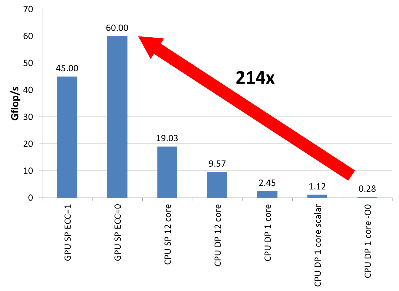
Blame the wimpy hardware: For multi- or many-core chips, per-core or per-thread metrics mask the inherent bottlenecks and are great for bashing your competitors. For instance, when comparing a multi-core CPU with a GPGPU you could declare that “the available bandwidth per thread is 122 times higher on the CPU than on the GPGPU.” Oh wait – make that 121.68 times.

taskmgr.png

Figure 1: Windows task manager is your friend: Four cores, all of them 100% utilized – that’s performance!

Boast frantic activity: MIPS (millions of instructions per second) or, equivalently, IPC (instructions per cycle) are perfect higher-is-better metrics if true performance is low. IPC can be boosted on purpose by several means: You can use a highly abstracting language to make the compiler generate a vast amount of instructions for simple things like loading a value from memory, or disable SIMD so that more instructions are executed for the same amount of work. Waiting in OpenMP barriers or MPI functions is also good for a large IPC count, since it often involves spin-waiting loops. You can use special options to disable compiler optimizations which have the potential to change numerical results (such as common subexpression elimination). But take care: If that means moving slow operations like floating-point divides into an inner loop, the IPC value will go down dramatically.

Fight the evil: State that your new code or new algorithm shows a factor of X fewer cache misses compared to the baseline. Cache misses are the black plague of HPC, so nobody will doubt your success. And they are just as easy to manipulate as Flops. Combining with the “go green” strategy is straightforward: Cache misses cost vast amounts of energy (they say), so you can be green and good at the same time!

Wow the management: State that “all processors are 100% utilized, so the code makes perfect use of the available resources.” Windows task manager is the perfect tool to show off with a stunt like this (see Fig. 1), but “top” under Linux works fine, too:

  PID VIRT RES  SHR %CPU %MEM  TIME+  P COMMAND 
 2318 492m 457m 596 98.6 22.9 0:35.52 2 a.out 
 2319 492m 457m 596 98.6 22.9 0:35.53 0 a.out 
 2321 492m 457m 596 98.6 22.9 0:35.50 1 a.out 
 2320 492m 457m 596 97.6 22.9 0:35.44 3 a.out

In summary, metrics are your wishing well: Find the right metric and any code will look good.

This stunt is essentially #9 of Bailey’s original “Twelve ways to fool the masses.”

Fooling the masses – Stunt 11: Show data! Plenty. And then some.

(See the prelude for some general information on what this is all about)

ShowDataPlenty_Bars

Figure 1: Lots of variants of an experiment, lots of machines, no idea for interpretation – why not show it all?

Computers produce data. Parallel computers produce more data. And doing performance experiments with parallel computers produces even more data, since we often conduct several runs with different code variants on different machines. Now imagine a situation where you’ve got all this data lying around on your disk, but you can’t make any sense of it. Since you wouldn’t bother to establish even a coarse performance model (your setup is just too complex for this kind of bean counting), you don’t know whether some particular performance measurement is “good” or “bad” on some particular machine, or how performance should change when some parameter is altered.

Why not put the cart before the horse and show all the data? This has decisive advantages: You can display all the work you did, without the embarrassing message that five or six numbers is all the relevant data you got from your research. Furthermore, it gives you the opportunity to add “discussion” at any desirable level of detail. For instance, if the page limit for submitting to your favorite conference is ten pages, and you have five pages full of messy bar graphs (such as the one shown in Fig. 1), you can easily fill the rest with meaningless “explanations” like “Variant 11 shows about 90% performance advantage on Machine G over Variant 10 on Machine F while, surprisingly, Variant 9 on Machine A is 6% slower than Variant 7 on Machine C.” You may want to write “92.23%” and “5.982%” here – see Stunt 8 for the reason.

In Summary, you can make up for your lack of insight by showing data. Plenty of it. Swamp your readers or your audience with hundreds of colorful bar graphs, scatter plots, timing diagrams, or whatever your favorite data visualization tool has to offer, and describe them at length. If you really want to leave the impression of true understanding, resort to obscure technical details − but this is the theme of another stunt.


Fooling the masses – Stunt 10: Always emphasize the “interesting” part of your work!

(See the prelude for some general information on what this is all about)

Have you ever thought about how to improve the aerodynamic properties of bulldozers? Yes? Then this stunt is for you.

Bulldozer aeodynamics

Figure 1: Always focus on the interesting stuff!

Code optimization is quite rewarding at times. You put all your effort into mutilating a chunk of code beyond all recognition, and in the end you get a 50% speedup. Often enough, this work requires a great deal of  expertise at the interface between hardware and software. And you certainly want to present your success to your peers so they understand how advanced you are.

If you do such a thing, don’t bother picking the low-hanging fruits. When 95% of the run time goes into a boring loop nest which multiplies a dense matrix with a vector, there is not much you can do beyond the standard textbook stuff – or use a library altogether. However, if the remaining 5% consist of a convoluted communication scheme, you’ve found your target. The fact that the possible gain is at most 5% shouldn’t stop you, because it’s all a matter of presentation; see Fig. 1: 3D bars and a proper choice of scales on the axes guide the reader’s eye and help you drive home your point. It’s like presenting the optimized drag coefficient of your aerodynamically improved bulldozer on high gloss paper, and the boring technical data in small black print on a dark blue background, on the back page.

Interestingly, if the optimization target is communication, or synchronization, or any other non-computational overhead, this stunt can be made to work even better: When you strongly scale to a pointless number of workers, reducing such overheads will give you arbitrary speedups, far beyond the factor of two that is theoretically possible if you restrict yourself to a sensible minimum parallel efficiency of 50%. Coming back to the heavy gear analogy, if you accelerate your bulldozer to 200 mph, the drag coefficient does become essential, and you may feel vindicated. It won’t solve any real-world problem, but hey, this is research after all.

Thanks to Gerhard Wellein for discovering this stunt in a paper. Many papers, actually.

Fooling the masses – Stunt 9: Boast massive speedups with accelerators!

(See the prelude for some general information on what this is all about)

GPGPUs, FPGAs, massively parallel single-chip multiprocessors: Accelerators are cool. The  prospect of boosting your application’s performance by 100x or more is mouthwatering, so you invest days and weeks, even months to port and tweak code and make it run fast on that shiny new piece of hardware. However, in the end the outcome may well be a meager 2.5x, or even much less, if you compare to well-optimized parallel code on a standard 2-socket server that everyone can handle.

What happened? Well, a direct peak performance and memory bandwidth comparison reveals that – even without considering Amdahl’s Law and overheads like PCIe transfers – 2x-4x is just what can be expected. Assuming a fair game, of course. And that’s exactly your chance to sugarcoat your mediocre results and fabricate a blazing success! Here are some hints:

  • Compare bleeding-edge accelerator technology with vintage CPUs. A Pentium III will be fine for most purposes today. If you can’t get your hands on one of those, give me a call.
  • Always compare the fully parallel accelerator code with a sequential (single-core) CPU version. You can even argue in favor of this, saying that “serial CPU code constitutes a well-defined baseline.” Be sure to rush ahead to the next slide before anyone dares to ask why you don’t use a single GPGPU “core” to make the comparison even more “well-defined.”
  • Use no optimizations whatsoever with the CPU compiler; -O0 will be fine. Also use a plain, proof-of-concept implementation of your algorithm with no manual code changes. It’s good scientific practice because a rock-bottom baseline is more meaningful!
  • Use single precision on the GPU but double precision on the CPU. That will effectively cut the CPU’s cache, the memory bandwidth, and its peak performance in half.
  • Accelerate only the kernels that are easily portable and report only their performance. Amdahl’s Law and communication overhead will be nothing but smoke and mirrors!
dens MVM GPU vs. CPU

Figure 1: If you do it right, a 200x speedup for the GPU is absolutely feasible (comparing nVIDIA Tesla C2050 and Intel Dual Xeon 5650, dense matrix-vector multiply, matrix size 4500×4500, Intel compiler V12 update 11)

These tricks should give you a competitive edge; 20x-200x reported speedup should be no problem, depending on your unscrupulousness.

See Fig. 1 for an instructive example: A dense matrix-vector multiply using a 4500×4500 matrix is memory-bound on a Fermi-type GPGPU as well as on a standard CPU-based system such as a dual-socket Xeon 5650 (“Westmere”). The GPGPU baseline of about 45 GFlop/s at single precision (SP) is completely in line with the achievable memory bandwidth of roughly 90 GB/s (4 bytes per multiply-add operation, assuming the right-hand side is mostly held in shared memory). To get a slight speedup you can switch off ECC (who cares for some flipped bits?) to get about 120 GB/s, corresponding to 60 GFlop/s. No need to mention that the PCIe transfers to get the RHS and result vectors to and from the device are neglected. So much for the GPGPU.

On the CPU side, the full dual-Xeon node has a bandwidth of close to 40 GB/s, leading to an SP performance of 19 GFlop/s – much too fast to be shown in public! Going to double precision cuts that in half, but there is more: Using just a single core gets you down another factor of 4, and disabling vectorization gives you a further 0.5x (since you’re now far away from any bandwidth limitation). Finally, turning off optimization altogether (-O0) lets you hit rock bottom at 248 MFlop/s – a whopping 214x slower than the best GPGPU result! Going to my old P-III is not even necessary any more.

Note the cunning use of a linear scale in the diagram; in this particular case it is much better than a log scale since it reduces the CPU performance “baseline” to a mere flyspeck (see Stunt 3 for more information on log vs. linear scale).

This stunt is essentially identical to #6 and #7 of Bailey’s original collection.

Fooling the masses – Stunt 8: Impress your audience with awe-inspiring accuracy

(See the prelude for some general information on what this is all about)

“Qualitative” statements make you cringe. Being a scientist, you know that science is all about accuracy. And what could be more accurate than numbers?  Good for you! There is ample opportunity for generating numbers in computer science. The art is to not block your audience’s view on the raw and unfiltered truth.

# cores Time (plain) [s] Time (optimized) [s] Speedup [%]
1 12.0435766 8.6198441 39.71919283
2 6.1179025 5.5901951 9.439874469
3 4.9041394 4.6966098 4.418710705
4 4.7002801 4.6912042 0.193466317

Fig. 1: Awesome! Up to 1.77992 times faster!

A simple example: When comparing performance numbers between different machines or code versions (see Stunt 7 for some amazing tricks you can play there), don’t hesitate to provide timings with sub-microsecond resolution, even if the results fluctuate like mad. Then state, in a slightly generalizing, “management-style” demeanor, that your “optimizations lead to a performance increase of up to 39.71919283%”, and refer to the data (see the table) to substantiate your assertion. In other words, forget what your high school teachers told you about significant digits and use the full power of your pocket calculator, even if a slide rule would also do the trick.

By the way, the same works for drawing conclusions from data in diagrams. Since it is sometimes hard to read off precise values from graphs, help your audience by stating the raw facts (see Fig. 1). Using boldface and jazzy colors will help to keep peoples’ attention on the important messages. Do not waste time and space dealing with lengthy explanations but let the numbers speak for themselves!


Fooling the masses – Stunt 7: Be creative when comparing scaled performance!

(See the prelude for some general information on what this is all about)

Scaling comparison

Fig. 1: Comparing performance vs. number of compute units (CPU sockets, GPUs) under limited scalability can yield any result if you do it right!

Strong scaling performance comparisons between standard (i.e., CPU-based) and accelerated (e.g., GPU-based) systems are particularly rewarding, since there is ample opportunity to generate any speedup number you want. It is not about fabricating a large GPU vs. CPU speedup – this special topic deserves its own stunt (stay tuned!). You can just as well apply it to a “baseline” vs. an “optimized” code on the same machine.

This may not be easy to digest on a theoretical level, so I explain it using an example: Assume we have a parallel CPU code whose strong scalability is limited by Amdahl’s Law with a serial runtime fraction of 0.3%. Hence, the speedup factor is limited to 333. A parallel GPGPU version of the same program achieves a speedup of 10 (compared to one CPU socket) for the parallel part, and of 5 for the sequential part. Figure 1 shows a performance comparison for up to 16384 compute units (CPU sockets or GPUs, respectively). As expected, the GPGPU speedup is 10 for small numbers of workers and goes down to 5 for large numbers – always comparing equal numbers of GPGPUs and CPU sockets. So far so good.

However, if you pose the right question, the factor can be much larger – even infinity, if you want: If we ask “How many CPU sockets do we need to outcompute 32 GPUs?”, the answer is clearly 2048. This means that your GPU-vs-CPU speedup is not 5, and also not 10, but almost 64 (see the dashed line in the graph). And its gets even better: Somewhere between 32 and 40 GPUs the required number of CPU sockets slips away to infinity! Your GPUs can go where no CPU has ever gone before (and never will)!

Efficiency comparison

Fig. 2: Plotting the parallel efficiency of both variants reveals the reason why the stunt works. Note that the efficiency of the GPU version is always worse.

The reason why this works is that you compare the two graphs at different numbers of workers – so different that the parallel efficiency for the CPU code is way down, whereas for the GPU code it is still acceptable (see Fig. 2)! Or to put it the other way round: If we compare equal numbers of workers on both sides, the parallel efficiency on the CPUs is always better.

The sensible way to compare achievable performance would be to set a certain practical lower limit for the parallel efficiency, e.g., 50%. From a computing center point of view, this is probably the lowest efficiency we’d be willing to accept, except in cases where the reason for going parallel is lack of memory. Scaling beyond that point does not make sense, not even for the purpose of comparison! A reasonable question to ask would be “How much performance can I get from the two codes at their respective minimum acceptable efficiency point?”

So the gist of it is: When comparing scaled performance data, ask the right questions and be the hero of the day. And don’t talk about parallel efficiency, or people might ask why you are wasting precious CPU cycles…

Thanks to Gerhard for discovering this extraordinary stunt!


Fooling the masses – Stunt 6: Ignore affinity and topology issues!

AMD Epyc 7451 node

Fig. 1: A dual-socket AMD Epyc 7451 node with four “Zeppelin” dies per socket (eight ccNUMA domains per node). Each 8 MiB L3 cache is shared by three cores, i.e., half the die.

(See the prelude for some general information on what this is all about)

Real scientists are not bothered by details such as multicore, cache groups, ccNUMA, SMT, or network hierarchies. Those are just parts of a vicious plot to take the fun out of computing. Ignoring the associated issues like bandwidth bottlenecks, NUMA locality and contention penalties, file system buffer cache, synchronization overheads, etc., will make them go away.

If you present performance data and people ask specific questions about affinity and topology awareness, answer that it’s the OS’s or the compiler’s job, or the job of some auto-tuning framework, to care about those technicalities. Probably you can show off by proving that your code scales even though you run it without topology awareness; this can be easily achieved by applying Stunt 2 – just slow down code execution enough to make all overheads vanish.

If you run into problems like mysterious performance fluctuations, or performance being too low altogether (a direct but often ignored consequence of applying Stunt 2), blame the system administrators. Being lowly minions of top-achieving scientists like you, they will have the time to figure out what’s wrong with their hardware. If they tell you it’s all your fault, send a scathing e-mail to their boss and cc: your university president or company CTO, just for good measure. Finally, if all else fails, publish a paper at a high-profile conference stating that the hardware of manufacturer X shows horrible performance, especially together with compiler Y and library Z, and that the cluster you had access to was too small to get the results that you wanted in time. That’s why you are about to write a generous research proposal for a federal supercomputing facility. Anything less just won’t cut the mustard!


The 400x GPU speedup baloney

Recently, in the HPC services office…

(… phone rings …)

“Computing Center, HPC services. How can I help you?”

“Yes, High Performance Computing.”

“You want to use our GPGPU cluster? Great! The load on this baby could be higher anyway. It’s hard to believe, but people seem to avoid it like the plague (jovial laughter). Do you have a code that runs on GPUs already?”

“I see, the compiler should be able to handle this. But the code is SIMD vectorized for standard processors, right?”

“No, this has nothing to do with cell phones. SIMD means ‘Single Instruction Multiple Data,’ i.e., several operations can be performed on different operands with a single machine instruction. If that works, chances are that the program can be run efficiently on a GPU as well. After all, GPUs implement the SIMD principle quite extensively.”

“Hm? I think I don’t understand…”

“Ah, ok. No, you don’t have to learn assembly programming to do this. But you may have to think a little more about how the compiler looks at your code. Often you can help it by supplying additional information, like source directives. And of course you need to use a compiler that understands what SIMD is. Alas, the GNU compilers don’t have a clue about it, mostly. By the way, how  have you parallelized the code?”

“Um, no. Compilers can’t help you much here, except for very simple cases where a 10-year-old can do it just as well. But you do have to parallelize. How do you want to draw a meaningful comparison to the GPU version?”

“What do you mean, you don’t need to do this?”

“Um, yes, I think I’ve seen this paper recently. It should be on my desk somewhere… (paper rustling) And what exactly are you referring to?”

“Section 4.3, just a sec… here we are: ‘As shown in Fig. whatever, we have achieved a 400x speedup on an NVIDIA Tesla GPU as compared with our CPU implementation.’ (long pause)”

“Sorry, no, I’m still here. I’ve just been looking for the details of the CPU implementation. One moment… (longer pause) Ok, here’s something in the caption of the pretty CFD visualization: ‘In order to avoid issues with OpenMP parallelization we have run the CPU version on a single core.’ Wow. This has to sink in. And if I’m not mistaken, they compare a single-precision GPU code with a double precision version on the CPU. Truly hilarious.”

“No, I’m not making fun of those scientists. But ‘scientists’ is not the word I would use. They obviously think that everyone else is stupid.”

“Why? Because a factor of 400 is impossible. Neither the floating-point peak performance nor the memory bandwidth of the GPU is 400 times larger than that of a current standard compute node, or a chip, or even a single core. So they must have fabricated a slow CPU code on purpose. Realistically one may expect a factor of 2-4 if you compare a reasonably optimized CPU code on a single node with a single GPU, and use the same precision on both.”

“Yes, I agree. 2-4 isn’t bad at all. But that’s just counting the raw GPU. How would the data transfer affect the performance of you code? Can you estimate this?”

“Well, somehow the data must be brought into the GPU and the results must be copied back so that they don’t start rotting over there…”

“Yes (sighing with resignation). Compilers are smart. But there are limits. If you copy the whole problem through the PCI bus after every step, the only way to exploit the performance advantage of the GPU is to perform ridiculously many flops. It’s all a matter of code balance.”

“Code balance tells you how much data transfer your code needs per executed floating-point operation – and you have to count everything, including communication via buses, the network, the memory interface, etc. This can add up to quite some data volume. And then you compare with the amount of data the hardware can transfer per peak flop executed, which gives you an estimate for the performance.”

“You don’t know how many flops and how much data transfer your code needs? Can’t you just count that by looking at it? In most cases, compute time is spent in a very limited number of numerical kernel loops.”

“No, the compiler doesn’t count that for you (keeping composure with obvious effort). It’s also a matter of optimization; perhaps one can reduce the data transfers a bit. One would have to take a look at the code.”

“The compiler? (devastated) Yes, you should try that. Definitely… No listen, people are much too enthusiastic about the compiler’s abilities. Compilers can not read your mind, they can’t even look through the standard C++ template tricks that programmers are so fond of. Let alone generate optimal code for GPUs.”

“Ok, err, sorry, are you crying? (nonplussed) Please don’t. May I suggest that we sit together over a cup of coffee and I give you a crash course in basic performance modeling? Don’t worry, everything’s going to be alright. There, there…”