[Update 17/11/29: Pointed out that the C version was modified from the original code – thanks Julian]
The Himeno benchmark [1] is a very popular code in the performance analysis and optimization community. Countless papers have been written that use it for performance assessment, prediction, optimization, comparisons, etc. Surprisingly, there is hardly a solid analysis of its data transfer properties. It’s a stencil code after all, and most of those can be easily analyzed.
The code
The OpenMP-parallel C version looks as shown below. I have made a slight change to the original code: The order of indices on the arrays a, b, and c hinders efficient SIMD vectorization, so I moved the short index to the first position. This also makes it equivalent to the Fortran version.
// all data structures hold single-precision values
for(n=0;n<nn;++n){
  gosa = 0.0;
  #pragma omp parallel for reduction(+:gosa) private(s0,ss,j,k)
  for(i=1 ; i<imax-1 ; ++i)
    for(j=1 ; j<jmax-1 ; ++j)
      for(k=1 ; k<kmax-1 ; ++k){
        // short index on a, b, c was moved up front
        s0 = a[0][i][j][k] * p[i+1][j ][k ]
           + a[1][i][j][k] * p[i ][j+1][k ]
           + a[2][i][j][k] * p[i ][j ][k+1]
           + b[0][i][j][k] * ( p[i+1][j+1][k ] - p[i+1][j-1][k ]
                             - p[i-1][j+1][k ] + p[i-1][j-1][k ] )
           + b[1][i][j][k] * ( p[i ][j+1][k+1] - p[i ][j-1][k+1]
                             - p[i ][j+1][k-1] + p[i ][j-1][k-1] )
           + b[2][i][j][k] * ( p[i+1][j ][k+1] - p[i-1][j ][k+1]
                             - p[i+1][j ][k-1] + p[i-1][j ][k-1] )
           + c[0][i][j][k] * p[i-1][j ][k ]
           + c[1][i][j][k] * p[i ][j-1][k ]
           + c[2][i][j][k] * p[i ][j ][k-1]
           + wrk1[i][j][k];
        ss = ( s0 * a[3][i][j][k] - p[i][j][k] ) * bnd[i][j][k];
        gosa = gosa + ss*ss;
        wrk2[i][j][k] = p[i][j][k] + omega * ss;
      }
  // copy-back loop ignored for analysis
  #pragma omp parallel for private(j,k)
  for(i=1 ; i<imax-1 ; ++i)
    for(j=1 ; j<jmax-1 ; ++j)
      for(k=1 ; k<kmax-1 ; ++k)
        p[i][j][k] = wrk2[i][j][k];
} /* end n loop */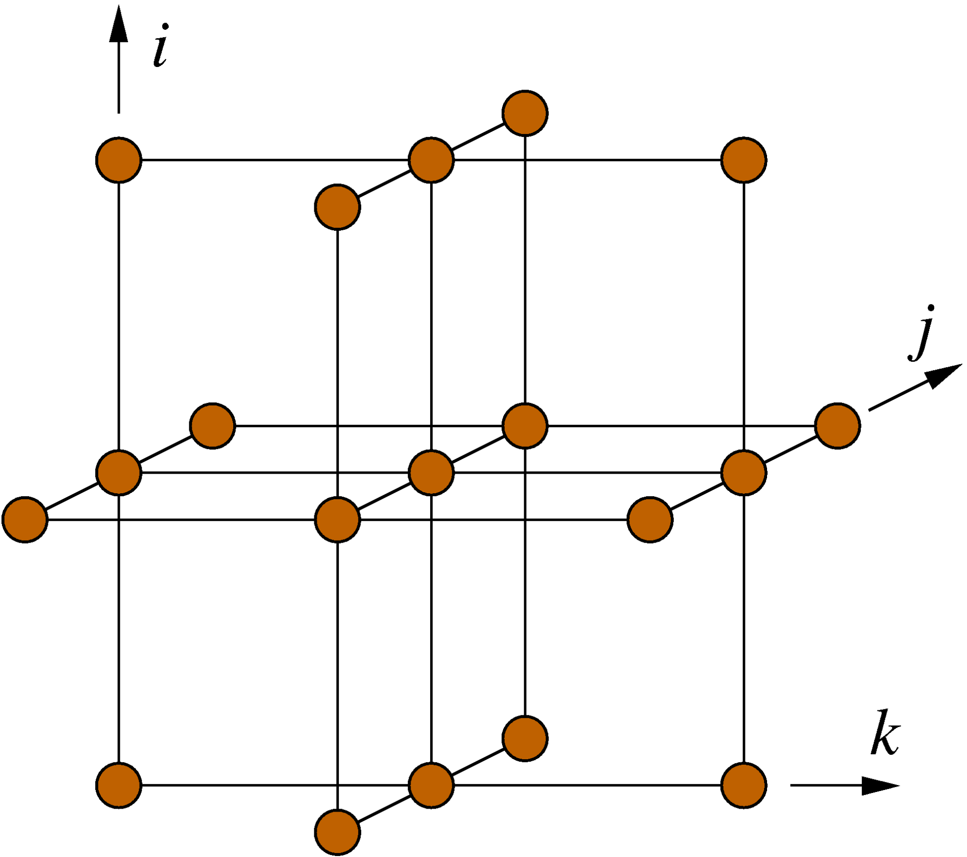
Figure 1: Structure of the 19-point stencil showing the data access pattern to the p[][][] array in the Himeno benchmark. The k index is the inner (fast) loop index here.
n. The first (parallel) loop nest over i, j, and k updates the wrk2 array from the arrays a, b, c, wrk1, bnd, and p, of which only p has a stencil-like access pattern (see Fig. 1). All others are accessed in a consecutive, cacheline-friendly way. Since the coefficient arrays a, b, and c carry a fourth index in the first position, the row-major data layout of the C language leads to many concurrent data streams. We will see whether or not this impacts the performance of the code.
A second parallel loop nest copies the result in wrk2 back to the stencil array p. This second loop can be easily optimized away (how?), so we ignore it in the following; all analysis and performance numbers pertain to the first loop only.
Amount of work
There are 14 floating-point additions, 7 subtractions, and 13 multiplications in the loop body. Hence, one lattice site update (LUP) amounts to 34 flops.
Data transfers and best-case code balance
For this analysis the working set shall be larger than any cache. It is straightforward to calculate a lower limit for the data transfers if we assume perfect spatial and temporal locality for all data accesses within one update sweep: All arrays except wrk2 must be read at least once, and wrk2 must be written. This leads to (13+1) single-precision floating-point numbers being transferred between the core(s) and main memory. The best-case code balance is thus Bc = 1.65 byte/flop = 56 byte/LUP. If the architecture has a write-back cache, an additional write-allocate transfer must be accounted for if it cannot be avoided (e.g., by nontemporal stores). In this case the best-case code balance is Bc = 1.76 byte/flop = 60 byte/LUP.
Considering that even the most balanced machines available today are not able to feed such a hunger for data (e.g., the new NEC-SX Aurora TSUBASA vector engine with 0.5 byte/flop), we know that this code will be memory bound. If the memory bandwidth can be saturated, the upper performance limit is the memory bandwidth divided by the code balance.