[Update 17/11/29: Pointed out that the C version was modified from the original code – thanks Julian]
The Himeno benchmark [1] is a very popular code in the performance analysis and optimization community. Countless papers have been written that use it for performance assessment, prediction, optimization, comparisons, etc. Surprisingly, there is hardly a solid analysis of its data transfer properties. It’s a stencil code after all, and most of those can be easily analyzed.
The code
The OpenMP-parallel C version looks as shown below. I have made a slight change to the original code: The order of indices on the arrays a, b, and c hinders efficient SIMD vectorization, so I moved the short index to the first position. This also makes it equivalent to the Fortran version.
// all data structures hold single-precision values
for(n=0;n<nn;++n){
  gosa = 0.0;
  #pragma omp parallel for reduction(+:gosa) private(s0,ss,j,k)
  for(i=1 ; i<imax-1 ; ++i)
    for(j=1 ; j<jmax-1 ; ++j)
      for(k=1 ; k<kmax-1 ; ++k){
        // short index on a, b, c was moved up front
        s0 = a[0][i][j][k] * p[i+1][j ][k ]
           + a[1][i][j][k] * p[i ][j+1][k ]
           + a[2][i][j][k] * p[i ][j ][k+1]
           + b[0][i][j][k] * ( p[i+1][j+1][k ] - p[i+1][j-1][k ]
                             - p[i-1][j+1][k ] + p[i-1][j-1][k ] )
           + b[1][i][j][k] * ( p[i ][j+1][k+1] - p[i ][j-1][k+1]
                             - p[i ][j+1][k-1] + p[i ][j-1][k-1] )
           + b[2][i][j][k] * ( p[i+1][j ][k+1] - p[i-1][j ][k+1]
                             - p[i+1][j ][k-1] + p[i-1][j ][k-1] )
           + c[0][i][j][k] * p[i-1][j ][k ]
           + c[1][i][j][k] * p[i ][j-1][k ]
           + c[2][i][j][k] * p[i ][j ][k-1]
           + wrk1[i][j][k];
        ss = ( s0 * a[3][i][j][k] - p[i][j][k] ) * bnd[i][j][k];
        gosa = gosa + ss*ss;
        wrk2[i][j][k] = p[i][j][k] + omega * ss;
      }
  // copy-back loop ignored for analysis
  #pragma omp parallel for private(j,k)
  for(i=1 ; i<imax-1 ; ++i)
    for(j=1 ; j<jmax-1 ; ++j)
      for(k=1 ; k<kmax-1 ; ++k)
        p[i][j][k] = wrk2[i][j][k];
} /* end n loop */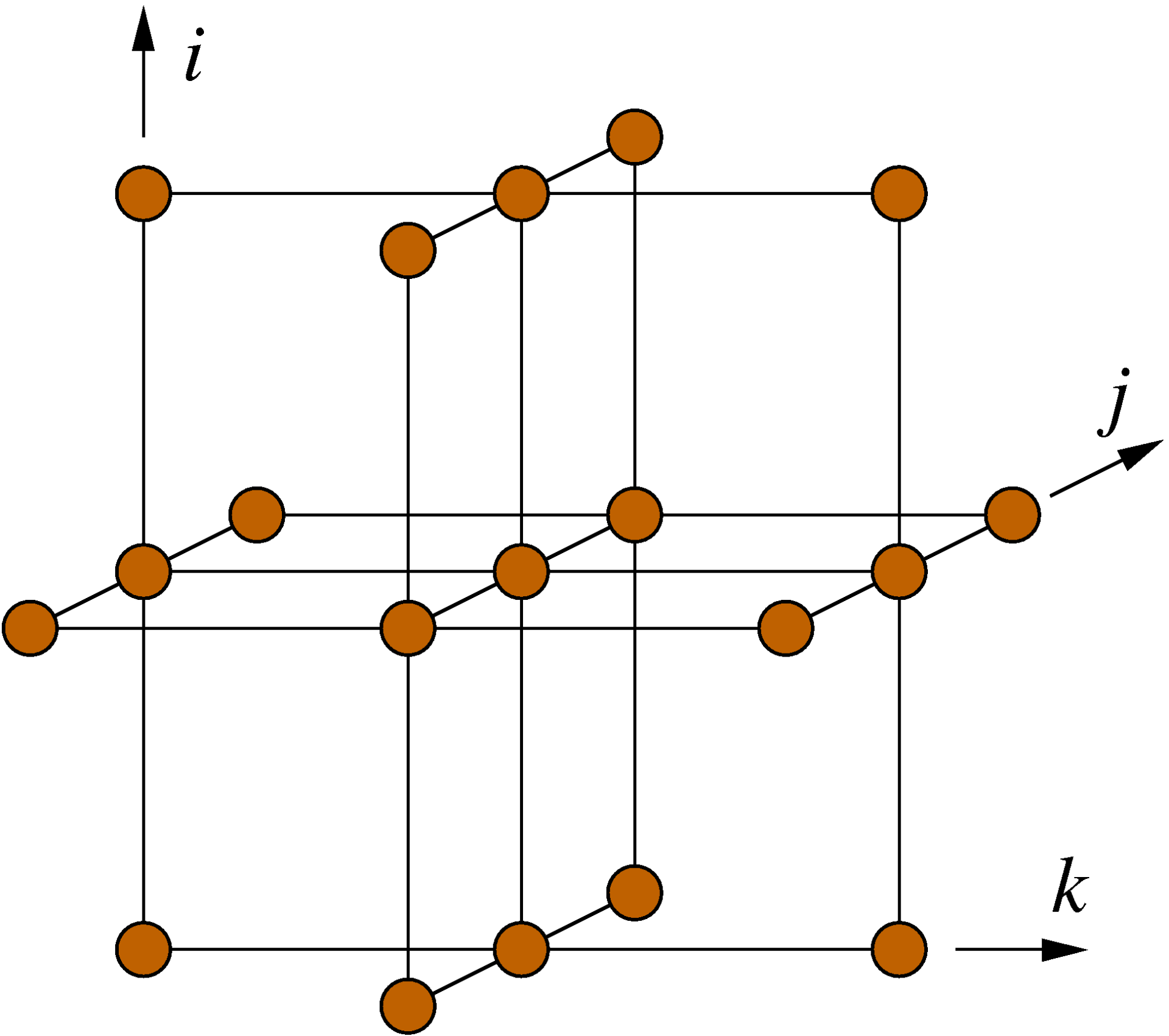
Figure 1: Structure of the 19-point stencil showing the data access pattern to the p[][][] array in the Himeno benchmark. The k index is the inner (fast) loop index here.
n. The first (parallel) loop nest over i, j, and k updates the wrk2 array from the arrays a, b, c, wrk1, bnd, and p, of which only p has a stencil-like access pattern (see Fig. 1). All others are accessed in a consecutive, cacheline-friendly way. Since the coefficient arrays a, b, and c carry a fourth index in the first position, the row-major data layout of the C language leads to many concurrent data streams. We will see whether or not this impacts the performance of the code.
A second parallel loop nest copies the result in wrk2 back to the stencil array p. This second loop can be easily optimized away (how?), so we ignore it in the following; all analysis and performance numbers pertain to the first loop only.
Amount of work
There are 14 floating-point additions, 7 subtractions, and 13 multiplications in the loop body. Hence, one lattice site update (LUP) amounts to 34 flops.
Data transfers and best-case code balance
For this analysis the working set shall be larger than any cache. It is straightforward to calculate a lower limit for the data transfers if we assume perfect spatial and temporal locality for all data accesses within one update sweep: All arrays except wrk2 must be read at least once, and wrk2 must be written. This leads to (13+1) single-precision floating-point numbers being transferred between the core(s) and main memory. The best-case code balance is thus Bc = 1.65 byte/flop = 56 byte/LUP. If the architecture has a write-back cache, an additional write-allocate transfer must be accounted for if it cannot be avoided (e.g., by nontemporal stores). In this case the best-case code balance is Bc = 1.76 byte/flop = 60 byte/LUP.
Considering that even the most balanced machines available today are not able to feed such a hunger for data (e.g., the new NEC-SX Aurora TSUBASA vector engine with 0.5 byte/flop), we know that this code will be memory bound. If the memory bandwidth can be saturated, the upper performance limit is the memory bandwidth divided by the code balance.
Layer conditions
If you know your stencils, you also know that this is not the whole story. The best-case code balance is calculated under the assumption that only one of all the accesses to the stencil array p, in this case one out of 19, actually goes to main memory. The rest can be reused from some level of cache. If this is true, and how much data must be supplied by the different memory hierarchy levels, can be determined by layer conditions (LCs). The outer (“3D”) layer condition is satisfied for the Himeno stencil if three j-k layers fit into the cache, i.e., 3\times 4\,\text{bytes}\times \mathtt{jmax}\times\mathtt{kmax} <C_\mathrm{eff}~, where C_\mathrm{eff} is an effective cache size; as a rule of thumb we can use half the available cache size per thread here (remember that the LC must be satisfied for each thread separately if static OpenMP scheduling is used). The middle (“2D”) layer condition is satisfied if nine inner rows of size kmax fit into the cache, i.e., three per j-k layer: 3\times 3\times 4\,\text{bytes} \times\mathtt{kmax}<C_\mathrm{eff}~.Finally, the inner (“1D”) layer condition requires that the cache can hold enough data to avoid cache misses on all but the “first” (largest k) accesses in the loop body. Even the L1 cache can do this for a radius-1 stencil like Himeno, so we don’t have to consider it here.
On processors with three cache levels, each of the LCs can be broken in any cache level, so there are actually nine layer conditions. Luckily, in a lowest-order analysis we are only interested in the memory traffic, so all we need to know is whether the most stringent LC is satisfied at the largest cache. In the Himeno case this is the 3D LC at L3. If it is broken, two additional data streams go out to memory, so the best-case code balance (with NT stores) rises to Bc= 64 byte/LUP = 1.88 byte/flop. If the memory bandwidth stays the same, the performance will thus go down by 12.5%. This is also the potential performance loss if spatial blocking is not done to establish the outer LC at L3. If NT stores are not used, the loss is even a little smaller. Here we see why spatial blocking for Himeno does not really pay off: The coefficient arrays dominate the data traffic, and the only relevant LC for the stencil array at the L3 cache at the problem default memory-bound sizes is the 3D LC.
The following table shows the predefined problem sizes in the Himeno benchmark, their working set sizes, and how much cache is needed per thread to satisfy the 3D LC:
| Problem size | imax x jmax x kmax |
Working set [MiB] | required cache per thread for 3D LC [MiB] |
| s | 129 x 65 x 65 | 29.1 | 0.048 |
| m | 257 x 129 x 129 | 228 | 0.19 |
| l | 513 x 257 x 257 | 1810 | 0.76 |
| xl | 1025 x 513 x 513 | 14406 | 3.0 |
Only the “xl” and “l” problems have the potential for breaking the 3D layer condition in the outermost cache. Hence, we expect roughly the same performance for “s” and “m”, and about 12% less for “l” and “xl”. The “s” problem may even fit into the cache on bigger CPUs, so we ignore it in the following. Using spatial blocking on the “xl” and “l” problems will get us only to the level of “m” and no further.
Roofline model and validation
In order to validate the model we have to run the code on a specific architecture. A 14-core Intel Xeon “Haswell” E5-2695v3 (2.30 GHz base clock frequency) has a shared L3 cache of 35 MiB if Cluster on Die (CoD) is not activated. 14 threads will easily break the 3D layer condition on the “xl” case, but what about “l”? 0.75 MiB per thread only add up to 10.5 MiB overall, which is smaller than half the L3 cache. This rule-of-thumb calculation may be OK for simple stencil codes where only two arrays are involved, but with the Himeno benchmark we have 16 data streams fighting for the cache space (3 for p and 13 for the other arrays). We should thus only expect to have 3/16 of the cache available for the three layers of p, and so the “l” case is also expected to violate the 3D LC in L3. The standard benchmark that best fits the data access characteristics of Himeno is the Schönauer Vector Triad (a[:]=b[:]+c[:]*d[:]), which on our machine yields a memory bandwidth of b=55.1 GB/s (measured with likwid-bench). The following table shows the expected code balance, upper performance limits, and measured performance (with 14 cores) for the three sizes on one socket:
| Problem size | Bc [byte/flop] ([byte/LUP]) | b/Bc [Gflop/s] ([MLUP/s]) | Measured perf. [Gflop/s] ([MLUP/s]) | Measured Bc [byte/LUP] |
| m | 1.76 (60) | 31.3 (921) | 31.6 (929) | 58.3 |
| l | 2.0 (68) | 27.6 (812) | 28.5 (838) | 66.6 |
| xl | 2.0 (68) | 27.6 (812) | 28.8 (847) | 67.6 |
The measured performance is slightly above the predictions because this processor has a large spread in memory bandwidth depending on the number of read streams vs. write streams: The more data is read (relatively speaking), the higher the bandwidth (with a load-only benchmark the memory bandwidth is about 63 GB/s). Since Himeno has 14 or 16 read streams (including the write-allocate) vs. a single write stream, it can be expected that the vector triad shows less saturated bandwidth. The sheer number of streams, which gets multiplied by the number of threads, is obviously not hazardous in this case.
In order to be really sure about our model (it could be just coincidence after all) we have to validate the data traffic expectations by direct measurement. The last column of the table above shows the measured (via likwid-perfctr) memory data traffic per LUP. The values are quite close to the prediction, which shows that our overall picture of what is going on here is correct.
No spatial blocking strategy whatsoever on any of the “m”, “l” and “xl” problem sizes will get us beyond the 32-ish Gflop/s for the “m” case, because this is where the code balance is at its minimum. This is why the Himeno benchmark code is so resistant to the standard auto-tuning strategies, unless they include temporal blocking. Julian’s online Layer Condition Calculator allows you to study layer conditions and optimal block sizes for arbitrary stencils.
Of course, there are some residual questions one may ask:
- What about single-core performance and scalability? To analyze this in detail we will need the ECM performance model, which should yield an accurate single-core performance prediction, including the significance of layer conditions on inner cache levels. This is something for a later post.
- Is it at all important whether or not the compiler vectorizes the code? It is for sure vectorizable, and the Intel compiler (at least) does it, but is it necessary? Here, too, the ECM model should give a hint.
- What about temporal blocking? Without the ECM model analysis, the expected speedup from temporal blocking is hard to estimate, but at least the memory-boundedness should be lifted.
- Would it make sense to change the data layout? The original C version has a different index ordering on the coefficient arrays, which makes vectorization much harder because those arrays are then non-consecutive in the inner loop dimension. On the other hand, this ordering reduces the number of concurrent data streams. As the above analysis shows, we are pretty much at the memory bandwidth limit, so the number of streams itself does not seem to be a big problem.
[1] http://accc.riken.jp/en/supercom/himenobmt, download at http://accc.riken.jp/en/supercom/himenobmt/download/98-source/