 In a previous post I have shown how to construct and validate a Roofline performance model for the Himeno benchmark. The relevant findings were:
- The Himeno benchmark is a rather standard stencil code that is amenable to the well-known layer condition analysis. For in-memory data sets it achieves a performance that is well described by the Roofline model.
- The performance potential of spatial blocking is limited to about 10% in the saturated case (on a Haswell-EP socket), because the data transfers are dominated by coefficient arrays with no temporal reuse.
- The large number of concurrent data streams through the cache hierarchy and into memory does not hurt the performance, at least not too much. We had chosen a version of the code which was easy to vectorize but had a lot of parallel data streams (at least 15, probably more if layer conditions are broken).
Some further questions pop up if you want more insight: Is SIMD vectorization relevant at all? Does the data layout matter? What is the single-core performance in relation to the saturated performance, and why? All these questions can be answered by a detailed ECM model, and this is what we are going to do here. This is a long post, so I provide some links to the sections below:
- Hardware and code
- In-core model
- Layer conditions and data transfers
- ECM model
- Performance check
- Saturation behavior
- Miscellaneous
Hardware and code
I will assume that the reader is familiar with stencil analysis, layer conditions, and the ECM model for Intel x86 CPUs. A nice intro to the ECM model in the context of stencil codes is given in [1]. You should also read my post about the Roofline model for Himeno. Most of the manual analysis below was double-checked with our kerncraft tool for automatic loop performance modeling and benchmarking [3].
We start with the same code as in the Roofline analysis: C with SIMD-friendly data layout (in contrast to the original code). This is the hardware:
- Xeon Haswell E5-2695v3, CoD mode, 14 cores per socket (7 per ccNUMA domain)
- Cache sizes: 32 KiB L1 per core, 256 KiB L2 per core, 17.5 MiB shared L3 for 7 cores
- Memory bandwidth per ccNUMA domain: 28.1 GB/s with Schönauer vector triad
(measured with likwid-bench) - Clock frequency (core and Uncore) fixed to 2.3 GHz via likwid-setFrequencies. Forgetting to fix the Uncore clock speed is a frequent source of errors in benchmarking modern Intel CPUs. The separate Uncore clock domain exists since Haswell.
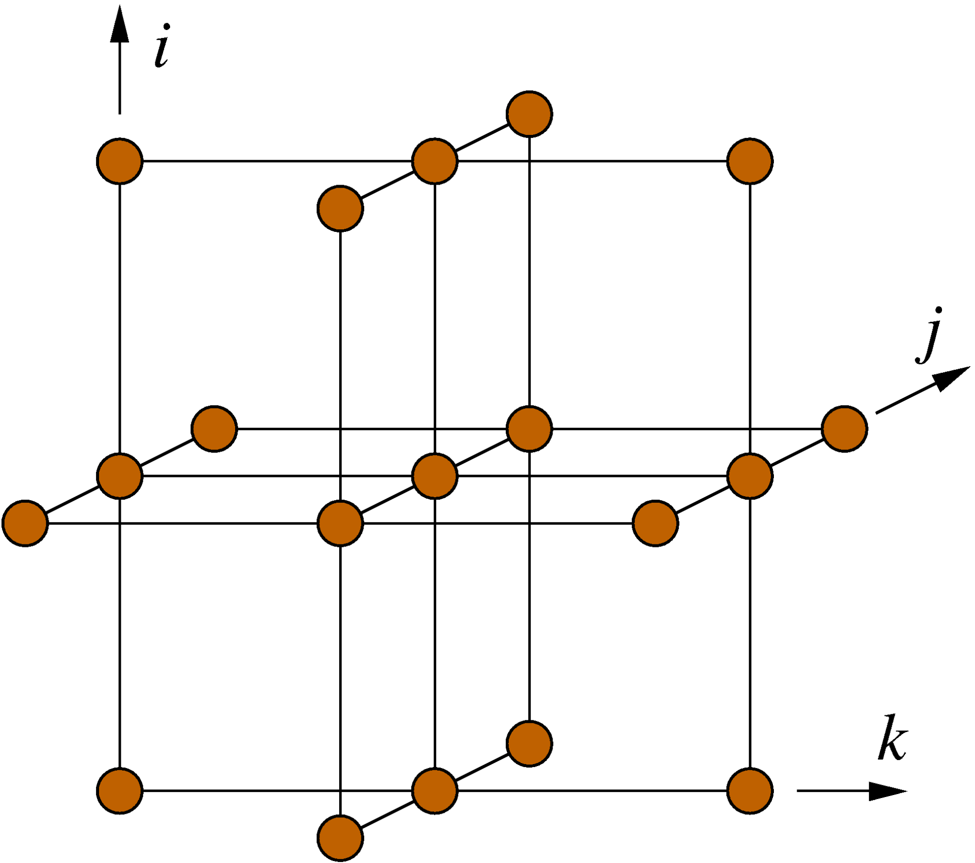
As before, we only look at the main loop and ignore the copy-back part, since that can be easily eliminated. The center loop nest is the following:
// SIMD-friendly data layout
for(int i=1 ; i<imax-1 ; ++i)
  for(int j=1 ; j<jmax-1 ; ++j)
    for(int k=1 ; k<kmax-1 ; ++k){
      // short index on a, b, c was moved up front
      s0 = a[0][i][j][k] * p[i+1][j ][k ]
         + a[1][i][j][k] * p[i ][j+1][k ]
         + a[2][i][j][k] * p[i ][j ][k+1]
         + b[0][i][j][k] * ( p[i+1][j+1][k ] - p[i+1][j-1][k ]
                           - p[i-1][j+1][k ] + p[i-1][j-1][k ] )
         + b[1][i][j][k] * ( p[i ][j+1][k+1] - p[i ][j-1][k+1]
                           - p[i ][j+1][k-1] + p[i ][j-1][k-1] )
         + b[2][i][j][k] * ( p[i+1][j ][k+1] - p[i-1][j ][k+1]
                           - p[i+1][j ][k-1] + p[i-1][j ][k-1] )
         + c[0][i][j][k] * p[i-1][j ][k ]
         + c[1][i][j][k] * p[i ][j-1][k ]
         + c[2][i][j][k] * p[i ][j ][k-1]
         + wrk1[i][j][k];
      ss = ( s0 * a[3][i][j][k] - p[i][j][k] ) * bnd[i][j][k];
      gosa = gosa + ss*ss;
      wrk2[i][j][k] = p[i][j][k] + omega * ss;
    }
The inner loop index k is also the last index on all arrays, which makes SIMD vectorization rather easy. If the short index on the arrays a, b, and c is moved to the back, this is more of a challenge since the accesses to those now become strided with respect to the inner loop index:
// SIMD-unfriendly data layout
for(int i=1 ; i<imax-1 ; ++i)
  for(int j=1 ; j<jmax-1 ; ++j)
    for(int k=1 ; k<kmax-1 ; ++k){
      // short index on a, b, c in original position
      s0 = a[i][j][k][0] * p[i+1][j ][k ]
         + a[i][j][k][1] * p[i ][j+1][k ]
         + a[i][j][k][2] * p[i ][j ][k+1]
         + b[i][j][k][0] * ( p[i+1][j+1][k ] - p[i+1][j-1][k ]
                           - p[i-1][j+1][k ] + p[i-1][j-1][k ] )
         + b[i][j][k][1] * ( p[i ][j+1][k+1] - p[i ][j-1][k+1]
                           - p[i ][j+1][k-1] + p[i ][j-1][k-1] )
         + b[i][j][k][2] * ( p[i+1][j ][k+1] - p[i-1][j ][k+1]
                           - p[i+1][j ][k-1] + p[i-1][j ][k-1] )
         + c[i][j][k][0] * p[i-1][j ][k ]
         + c[i][j][k][1] * p[i ][j-1][k ]
         + c[i][j][k][2] * p[i ][j ][k-1]
         + wrk1[i][j][k];
      ss = ( s0 * a[i][j][k][3] - p[i][j][k] ) * bnd[i][j][k];
      gosa = gosa + ss*ss;
      wrk2[i][j][k] = p[i][j][k] + omega * ss;
    }
However, all cache lines are still fully used, so the Roofline model does not change (assuming everything is still strongly bandwidth bound). In the following analysis we will look at both code versions; as seen from the ECM model they do not differ in the data transfer volume but only in the in-core part.
In-core model
The kernel executes 13 multiplications and 21 additions or subtractions. Some of those are fused by the compiler into FMAs. Just by looking at the code we need 32 loads and one store, but the massive amount of memory references may lead to some spilling, presumably with registers holding array base addresses. This is the inner loop code that the Intel compiler generates for the SIMD-friendly code (version 17.0 Update 5, compile options -std=c99 -O3 -xCORE-AVX2 -fno-alias):
# SIMD-friendly layout (Intel 17.0up5)
mov r15, qword ptr [rsp+0x210]
vmovups ymm8, ymmword ptr [r10+r12*4+0x8]
vmovups ymm15, ymmword ptr [r9+r12*4+0x8]
vmovups ymm12, ymmword ptr [r15+r12*4+0x4]
vmovups ymm4, ymmword ptr [r13+r12*4+0x4]
vmovups ymm6, ymmword ptr [r10+r12*4+0x4]
vmovups ymm7, ymmword ptr [r14+r12*4+0x8]
vmovups ymm9, ymmword ptr [r9+r12*4+0x4]
vmovups ymm10, ymmword ptr [r14+r12*4+0x4]
vsubps ymm8, ymm8, ymmword ptr [rdi+r12*4+0x8]
vsubps ymm2, ymm15, ymmword ptr [r13+r12*4+0x8]
mov r15, qword ptr [rsp+0x1d0]
vsubps ymm3, ymm2, ymmword ptr [r9+r12*4]
vmovups ymm2, ymmword ptr [rdi+r12*4+0x4]
vsubps ymm13, ymm12, ymmword ptr [r15+r12*4+0x4]
vsubps ymm12, ymm8, ymmword ptr [r10+r12*4]
vaddps ymm3, ymm3, ymmword ptr [r13+r12*4]
vsubps ymm14, ymm13, ymmword ptr [r11+r12*4+0x4]
vaddps ymm13, ymm12, ymmword ptr [rdi+r12*4]
vmovups ymm8, ymmword ptr [rsi+r12*4+0x4]
mov r15, qword ptr [rsp+0x1d8]
vfmadd213ps ymm8, ymm4, ymmword ptr [rdx+r12*4+0x4]
vaddps ymm5, ymm14, ymmword ptr [r15+r12*4+0x4]
vmovups ymm14, ymmword ptr [rax+r12*4+0x4]
vmulps ymm5, ymm5, ymmword ptr [r8+r12*4+0x4]
vmulps ymm4, ymm14, ymmword ptr [r14+r12*4]
mov r15, qword ptr [rsp+0x1e8]
vfmadd231ps ymm8, ymm13, ymmword ptr [r15+r12*4+0x4]
mov r15, qword ptr [rsp+0x1f0]
vfmadd231ps ymm4, ymm2, ymmword ptr [r15+r12*4+0x4]
mov r15, qword ptr [rsp+0x1c8]
vaddps ymm15, ymm8, ymm4
vfmadd231ps ymm5, ymm6, ymmword ptr [r15+r12*4+0x4]
mov r15, qword ptr [rsp+0x1e0]
vmulps ymm6, ymm3, ymmword ptr [r15+r12*4+0x4]
mov r15, qword ptr [rsp+0x218]
vfmadd231ps ymm6, ymm7, ymmword ptr [r15+r12*4+0x4]
vaddps ymm7, ymm5, ymm6
nop
mov r15, qword ptr [rsp+0x220]
vfmadd231ps ymm7, ymm9, ymmword ptr [r15+r12*4+0x4]
mov r15, qword ptr [rsp+0x200]
vaddps ymm2, ymm7, ymm15
vmovups ymm9, ymmword ptr [r15+r12*4+0x4]
vfmsub213ps ymm9, ymm2, ymm10
vmulps ymm3, ymm9, ymmword ptr [rcx+r12*4+0x4]
vfmadd231ps ymm10, ymm1, ymm3
# this is the reduction on gosa
vfmadd231ps ymm11, ymm3, ymm3
vmovups ymmword ptr [rbx+r12*4+0x4], ymm10
add r12, 0x8
cmp r12, qword ptr [rsp+0x1b0]
jb 0xfffffffffffffeab
This is one full AVX iteration (eight scalar iterations). For some reason the compiler refrains from using half-wide LOAD instructions, which makes the code very clean. As expected, some integer register spill has occurred: Register r15 is loaded ten times from the stack, for an overall load count of 42. As for arithmetic, there are 13 FMA or multiply instructions and 12 add or subtract instructions in the assembly code.
For a full cache line (16 scalar iterations) we thus have a non-overlapping time of T_\mathrm{nOL}=42\,\text{cy} because the core can execute two loads per cycle. Just looking at the arithmetic, the 26 FMAs and 24 add/subtracts take 37 cycles, but we need 43 cycles to generate the necessary addresses. Hence, we have T_\mathrm{OL}=43\,\text{cy}. Intel IACA reports 46 cycles due to a backend stall. Close enough IMO. As long as T_\mathrm{nOL} and T_\mathrm{OL} are in the same ballpark, we know that the data delay will dominate anyway in the end.
This analysis assumes full instruction throughput, i.e., completely independent instructions that are fed to the execution ports as fast as they arrive. If you know your CPU architecture there is actually a little problem with that (highlighted in the assembly listing above): The sum reduction on the gosa variable causes a stall due to an inter-iteration dependency on register ymm11 . However, this little extra time can be easily hidden behind all the other stuff that’s going on in the kernel. In other words, it is not on the critical path.
How about the SIMD-unfriendly layout? The Intel compiler, in its unique way of doing everything it can to vectorize the code, generates pretty much the same arithmetic but has to account for scattered loads from the coefficient arrays:
# SIMD-unfriendly layout (Intel 17.0up5)
vmovups xmm7, xmmword ptr [rdx]
vmovups xmm10, xmmword ptr [rdx+0x10]
vmovups xmm13, xmmword ptr [rdx+0x20]
vmovups xmm5, xmmword ptr [rdx+0x30]
vmovups xmm15, xmmword ptr [rbx]
mov r15, qword ptr [rsp+0x1a8]
vinsertf128 ymm9, ymm7, xmmword ptr [rdx+0x40], 0x1
vinsertf128 ymm3, ymm10, xmmword ptr [rdx+0x50], 0x1
vinsertf128 ymm2, ymm13, xmmword ptr [rdx+0x60], 0x1
vinsertf128 ymm4, ymm5, xmmword ptr [rdx+0x70], 0x1
add rdx, 0x80
vshufps ymm7, ymm9, ymm3, 0x14
vshufps ymm14, ymm4, ymm2, 0x41
vshufps ymm6, ymm7, ymm14, 0x6c
vshufps ymm7, ymm7, ymm14, 0x39
vmovups xmm14, xmmword ptr [rbx+0x10]
vmovups xmm5, xmmword ptr [rbx+0x20]
vmovups ymm10, ymmword ptr [r9+r10*4+0x4]
vshufps ymm9, ymm9, ymm3, 0xbe
vshufps ymm0, ymm4, ymm2, 0xeb
vmovups ymm4, ymmword ptr [r14+r10*4+0x8]
vsubps ymm4, ymm4, ymmword ptr [r8+r10*4+0x8]
vsubps ymm4, ymm4, ymmword ptr [r14+r10*4]
vshufps ymm13, ymm9, ymm0, 0x6c
vshufps ymm9, ymm9, ymm0, 0x39
vmovups ymm0, ymmword ptr [rcx+r10*4+0x8]
vsubps ymm0, ymm0, ymmword ptr [rdi+r10*4+0x8]
vinsertf128 ymm12, ymm15, xmmword ptr [rbx+0x30], 0x1
vinsertf128 ymm3, ymm14, xmmword ptr [rbx+0x40], 0x1
vinsertf128 ymm5, ymm5, xmmword ptr [rbx+0x50], 0x1
add rbx, 0x60
vblendps ymm2, ymm3, ymm5, 0x22
vblendps ymm15, ymm12, ymm5, 0x44
vshufps ymm2, ymm12, ymm2, 0x6c
vshufps ymm14, ymm3, ymm15, 0x9c
vblendps ymm3, ymm12, ymm3, 0x22
vmovups ymm12, ymmword ptr [r15+r10*4+0x4]
vaddps ymm15, ymm4, ymmword ptr [r8+r10*4]
vsubps ymm4, ymm0, ymmword ptr [rcx+r10*4]
vmovups xmm0, xmmword ptr [rax]
vaddps ymm4, ymm4, ymmword ptr [rdi+r10*4]
vshufps ymm5, ymm3, ymm5, 0xc6
vsubps ymm3, ymm12, ymmword ptr [r13+r10*4+0x4]
mov r15, qword ptr [rsp+0x1b0]
vshufps ymm14, ymm14, ymm14, 0xd2
vmulps ymm14, ymm14, ymm15
vsubps ymm12, ymm3, ymmword ptr [r15+r10*4+0x4]
vmovups ymm3, ymmword ptr [r8+r10*4+0x4]
nop dword ptr [rax], eax
vfmadd132ps ymm13, ymm14, ymmword ptr [r9+r10*4+0x8]
vaddps ymm12, ymm12, ymmword ptr [r11+r10*4+0x4]
vmulps ymm2, ymm2, ymm12
vmovups xmm12, xmmword ptr [rax+0x10]
vfmadd132ps ymm6, ymm2, ymmword ptr [rcx+r10*4+0x4]
vmovups xmm2, xmmword ptr [rax+0x20]
vaddps ymm13, ymm6, ymm13
vfmadd132ps ymm7, ymm13, ymmword ptr [r14+r10*4+0x4]
mov r15, qword ptr [rsp+0x1b8]
vinsertf128 ymm12, ymm12, xmmword ptr [rax+0x40], 0x1
vinsertf128 ymm2, ymm2, xmmword ptr [rax+0x50], 0x1
vblendps ymm15, ymm12, ymm2, 0x22
vinsertf128 ymm0, ymm0, xmmword ptr [rax+0x30], 0x1
add rax, 0x60
vshufps ymm14, ymm0, ymm15, 0x6c
vblendps ymm15, ymm0, ymm2, 0x44
vshufps ymm6, ymm12, ymm15, 0x9c
vblendps ymm0, ymm0, ymm12, 0x22
vshufps ymm6, ymm6, ymm6, 0xd2
vshufps ymm2, ymm0, ymm2, 0xc6
vfmadd213ps ymm6, ymm3, ymmword ptr [rsi+r10*4+0x4]
vmulps ymm3, ymm2, ymmword ptr [r9+r10*4]
vfmadd213ps ymm5, ymm4, ymm6
nop
vfmadd132ps ymm14, ymm3, ymmword ptr [rdi+r10*4+0x4]
vaddps ymm4, ymm5, ymm14
vaddps ymm2, ymm7, ymm4
vfmsub213ps ymm9, ymm2, ymm10
vmulps ymm3, ymm9, ymmword ptr [r12+r10*4+0x4]
vfmadd231ps ymm10, ymm1, ymm3
vfmadd231ps ymm11, ymm3, ymm3
vmovups ymmword ptr [r15+r10*4+0x4], ymm10
add r10, 0x8
cmp r10, qword ptr [rsp+0x180]
jb 0xfffffffffffffe19
The extra “processor work” mainly consists of some half-wide loads and shuffles, which put some extra pressure on ports 0, 1, and 5, and leads to a slight increase in the overlapping time, which is now T_\mathrm{OL}=54.5\,\text{cy} according to IACA (frontend bottleneck due to several ports having similar load now). The non-overlapping time rises to a nondramatic T_\mathrm{nOL}=46\,\text{cy}; although the integer register spill was reduced (only 3 additional loads to r15 instead of 10), the half-wide loads come at an additional cost. All this shows that the “bad” data layout can be almost compensated by the ability of the architecture to move the complex shuffling and shifting between SIMD registers off the critical path. You need a good compiler, of course.
Speaking of compilers: I don’t want to turn this into a compiler shoot-out, but at least we have to throw a glance at what happens when the compiler cannot vectorize. Using gcc 7.2.0 and options -std=c99 -Ofast -mavx2 -mfma -fargument-noalias I got the following code with the SIMD-friendly data layout:
# scalar code for SIMD-friendly layout (gcc 7.2.0)
vmovss xmm1, dword ptr [r14+rax*4]
add r8, 0x4
add rdi, 0x4
mov r12, qword ptr [rbp-0x68]
vmovss xmm0, dword ptr [r15+rax*4]
vmulss xmm1, xmm1, dword ptr [rcx+0x4]
mov r9, qword ptr [rbp-0xa0]
add rdx, 0x4
vmulss xmm0, xmm0, dword ptr [rdi]
add rsi, 0x4
add rcx, 0x4
vmovss xmm2, dword ptr [r12+rax*4]
mov r12, qword ptr [rbp-0x60]
vmovss xmm4, dword ptr [r9+rax*4]
mov r9, qword ptr [rbp-0x90]
vmovss xmm3, dword ptr [r12+rax*4]
mov r12, qword ptr [rbp-0x98]
vfmadd132ss xmm2, xmm1, dword ptr [rdx+0x4]
vfmadd231ss xmm0, xmm3, dword ptr [r8]
vaddss xmm1, xmm2, xmm0
vmovss xmm0, dword ptr [r11+rax*4]
vmulss xmm0, xmm0, dword ptr [rdx-0x4]
vmovss xmm2, dword ptr [r12+rax*4]
mov r12, qword ptr [rbp-0x78]
vfmadd132ss xmm2, xmm0, dword ptr [rsi]
vaddss xmm0, xmm1, xmm2
vmovss xmm1, dword ptr [r10+rax*4]
vsubss xmm1, xmm1, dword ptr [rbx+rax*4]
vsubss xmm1, xmm1, dword ptr [r12+rax*4]
mov r12, qword ptr [rbp-0x80]
vaddss xmm1, xmm1, dword ptr [r12+rax*4]
mov r12, qword ptr [rbp-0x70]
vfmadd132ss xmm1, xmm4, dword ptr [r12+rax*4]
vaddss xmm1, xmm0, xmm1
vmovss xmm0, dword ptr [r8+0x4]
vsubss xmm0, xmm0, dword ptr [rcx+0x4]
vsubss xmm0, xmm0, dword ptr [r8-0x4]
vaddss xmm0, xmm0, dword ptr [rcx-0x4]
vmulss xmm2, xmm0, dword ptr [r9+rax*4]
vmovss xmm0, dword ptr [rdi+0x4]
vsubss xmm0, xmm0, dword ptr [rsi+0x4]
mov r9, qword ptr [rbp-0x88]
vsubss xmm0, xmm0, dword ptr [rdi-0x4]
vaddss xmm0, xmm0, dword ptr [rsi-0x4]
vfmadd132ss xmm0, xmm2, dword ptr [r9+rax*4]
vaddss xmm0, xmm1, xmm0
mov r9, qword ptr [rbp-0xa8]
vmovss dword ptr [rbp-0x40], xmm0
vmovss xmm5, dword ptr [rdx]
vfmsub132ss xmm0, xmm5, dword ptr [r13+rax*4]
vmulss xmm0, xmm0, dword ptr [r9+rax*4]
mov r9, qword ptr [rbp-0x58]
vmovaps xmm1, xmm0
vmovss dword ptr [rbp-0x44], xmm0
vfmadd213ss xmm1, xmm0, dword ptr [rbp-0x48]
vmovss dword ptr [rbp-0x48], xmm1
vmovss xmm6, dword ptr [rdx]
vfmadd132ss xmm0, xmm6, dword ptr [rbp-0x3c]
vmovss dword ptr [r9+rax*4], xmm0
add rax, 0x1
cmp rax, qword ptr [rbp-0xb0]
jnz 0xfffffffffffffec1
This is purely scalar code with no unrolling on top. The compiler, although it recognizes the architecture and employs FMA instructions, refuses to use any xmm register beyond xmm6, which leads to some more spills. We now have T_\mathrm{OL}=377\,\text{cy} and T_\mathrm{nOL}=370\,\text{cy}, a massive increase from either SIMD code shown above. We will see below whether or not this has any influence on the saturated performance.
Layer conditions and data transfers
Since we want an accurate single-core model we have to look at the data transfers through the complete memory hierarchy instead of just to and from main memory.
In order to keep it simple we start with a problem size around “xl” from the original Himeno set (xl has 513\times513 grid points in the inner two dimensions l and k). Looking at the cache sizes and the Roofline analysis we conclude that the 3D layer condition is satisfied in the L3 cache (and broken in L2 and L1), while the 2D layer condition is satisfied in L2 (and broken in L1). Why? The 2D layer condition requires to accommodate three rows of the array p per outer (i) layer in some cache. This data alone has a size of 513\times 3\times 3\times 4\,\text{byte}\approx 18\,\text{KiB}~, which is more than half the L1 cache size but fits easily into L2 even with all the other streams taking up cache space. The 3D layer condition requires 513\times 513\times 3\times 4\,\text{byte}\approx 3.0\,\text{MiB}~, which fits nicely into the 17.5 MiB L3 cache if only a single thread is running, but a parallel code with static scheduling of the outer loop will break the condition (as shown in the Roofline analysis). We will have to keep this in mind when we look at the scalability analysis.
Now we can write down the data transfer volumes between adjacent cache levels for one cacheline (16 iterations) of work: \{V_\mathrm{L1L2}\,|\,V_\mathrm{L2L3}\,|\,V_\mathrm{L3Mem}\}=\{23\,|\,17\,|\,15\}\,\text{CLs} The memory data volume will go up to 17 CLs if the 3D layer condition is broken due to shared cache shortage when running multiple threads.
ECM model
If you look into the Intel64 and IA-32 architectures optimization reference manual, and you’re lucky enough to find the right section about the Haswell architecture, then you find that Haswell can theoretically transfer one full cacheline per cycle between L1 and L2. Unfortunately, this is not what you measure in practice [2]. Of course the ECM model for Intel x86 architectures tells us that this bandwidth can never be observed in a benchmark because of the non-overlapping L1 cache, but even if you take this into account, Haswell can only manage to transfer 43 bytes/cy under best conditions (this has been corrected with Skylake, by the way). Hence, we will use a theoretical L1-L2 bandwidth of 43 bytes/cy here. For the memory bandwidth we use the upper limit of 28.12 GB/s measured with the Schönauer vector triad (triad_avx code from likwid-bench). The ccNUMA domain can actually deliver up to 32.4 GB/s in read-only mode, but since our machine model cannot describe those differences in saturated bandwidth we make it a little more “gray-box” and use a baseline benchmark that has a strong load/store ratio.
Translating the memory data volume into a number of cycles is simple. If V is the data volume in cache lines, b_\mathrm{S} is the memory bandwidth, and l is th cache line size in bytes, then the number of cycles is\frac{V\times l\times f}{b_\mathrm{S}}~,where f is the clock frequency in cycles per second.
SIMD-friendly layout, vectorized code (V1)
Using the input from above, the code with SIMD-friendly data layout has the following cycle counts for 16 scalar iterations: \{T_\mathrm{OL}\,\|\,T_\mathrm{nOL}\,|\,T_\mathrm{L1L2}\,|\,T_\mathrm{L2L3}\,|\,T_\mathrm{L3Mem}\}=\{43\,\|\,42\,|34.2\,|\,34\,|\,78.5\}\,\text{cy} Taking into account the non-overlapping machine model for Intel x86 CPUs we get an expected runtime of (42+34.2+34+78.5)\,\text{cy}\approx 189\,\text{cy}. The expected saturation point is at n_\mathrm{s}=\left\lceil \frac{189}{89}\right\rceil=3\,\text{cores}. The 89 cy come from the excess memory data volume due to the broken 3D LC in the L3 cache: 78.5\cdot\frac{17}{15}\approx 89.
SIMD-unfriendly layout, vectorized code (V2)
The flipped data layout has exactly the same data delay as the SIMD-friendly layout. The only thing that changes is the overlapping and non-overlapping time: \{T_\mathrm{OL}\,\|\,T_\mathrm{nOL}\,|\,T_\mathrm{L1L2}\,|\,T_\mathrm{L2L3}\,|\,T_\mathrm{L3Mem}\}=\{54.5\,\|\,46\,|34.2\,|\,34\,|\,78.5\}\,\text{cy} The resulting expected runtime is (46+34.2+34+78.5)\,\text{cy}\approx 193\,\text{cy}. We see that the increase in the overlapped time is irrelevant, and the only expected slowdown comes from the slightly larger number of loads in the loop kernel. However, the difference is only 2% and will hardly be noticeable. It is highly likely that other effects our model cannot encompass (like the change in the data access pattern) are more important. In short, the ECM model does not predict a significant change in performance for the SIMD-unfriendly data layout. The saturation point does not change either.
SIMD-friendly layout, scalar code (gcc) (V3)
We have seen above that gcc 7.2.0 did not produce the best possible scalar code (due to its sturdy refusal to use more than eight floating-point registers), but let’s use it anyway because it leads to an interesting corner case. We get\{T_\mathrm{OL}\,\|\,T_\mathrm{nOL}\,|\,T_\mathrm{L1L2}\,|\,T_\mathrm{L2L3}\,|\,T_\mathrm{L3Mem}\}=\{377\,\|\,370\,|34.2\,|\,34\,|\,78.5\}\,\text{cy}~.The kernel is obviously still data bound. The expected runtime is then (370+34.2+34+78.5)\,\text{cy}\approx 516\,\text{cy}, a 2.7\times slowdown compared to the best code. The saturation point is at n_\mathrm{s}=\left\lceil \frac{516}{89}\right\rceil=6\,\text{cores}, so we expect this code to just barely saturate within a ccNUMA domain (but experience shows that there will be less-than-perfect scalability since the memory bandwidth is still very close to saturation).
Peformance check
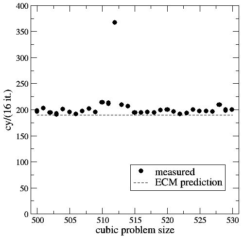
Figure 1: Serial runtime of 16 scalar iterations of version 1 versus problem size (cubic domain). Statistical variations of individual measurements were always below 1%.
Does the model predict the runtime or performance of the code accurately?
Unfortunately, if you set the xl problem size as defined in the original Himeno benchmark (1025\times513\times513), the model isn’t too accurate. In fact, the leading dimension seems dangerously close to a power of two, and if you play around with the sizes (including the outer size!) you see significant runtime variations. To explore this we set a cubic problem size of N\times N\times N and scan N from 500 to 530. The following benchmark data has been taken with the “Benchmark” mode of kerncraft. Individual measurements vary by less than 1% from run to run, so I didn’t include error bars.
Figure 1 shows the number of cycles for 16 iterations versus problem size for version 1 together with the ECM prediction of 190 cycles. Indeed, near a problem size of 512^3 the model is too optimistic. This might have been expected, especially for the SIMD-friendly data layout, since the neighbor accesses in the stencil and also the accesses to different components (first index) in the coefficient arrays a, b, and c have mutual distances of powers of two, or very close to that. The massive performance breakdown at N=512 speaks for itself.
On the bright side, the ECM model provides a very good prediction of the single-threaded runtime away from “pathological” cases. This experiment also shows that it is always good to look at performance numbers over a range of problem sizes. Figure 2 shows measurements for version 2 (SIMD code on SIMD-unfriendly data layout). Although there is a slight dip at N=512, the strong variations of runtime vs. problem size are mostly gone, because the index order on the coefficient arrays now causes an automatic skew in the access pattern. The only remaining issue is with the stencil array p. Although the ECM model is also accurate here with an error of well below 5%, our expectation that the code should be slightly slower than version 1 is not satisfied. On the contrary, the code is slightly faster. However, we have already mentioned above that the 2% of expected speedup can be easily swamped by other effects. We’ll come back to that later.
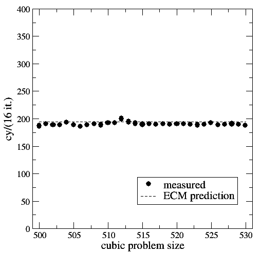
Figure 2: Serial runtime of 16 scalar iterations of version 2 versus problem size (cubic domain). Statistical variations of individual measurements were always below 1%.
Finally, Figure 3 shows measurements for version 3 (scalar gcc code on SIMD-friendly data layout). Again we see strong variations with problem size as with version 1, but the ECM model still yields a good prediction even in this very core-dominated case. The best measured value is 478 cy, which is 5.6% faster than the model prediction. This is not unexpected because we know that there is some overlap in the memory hierarchy when the in-core part is slow, even if it’s load dominated. 370 of the 516 predicted cycles are spent with loads in the core, but still the data delay down to memory accounts for a significant part of the runtime. The code is thus far from being totally “core dominated.”
Now what is the take-home message from all this? First of all, we have learned that the data layout has only a minor impact on the code performance as long as the code is vectorized. We could have found out about this just by taking the performance data, but thanks to the model we understand why: The major part of the execution time is still in the data delay, and even the in-core part is only changed slightly because all the “complicated” stuff that’s necessary to vectorize the code happens in the overlapping in-core part. This part with its 50-ish cycles hardly stretches beyond the L1 cache. Optimizing the SIMD code is difficult because the runtime is almost evenly spread across the whole memory hierarchy. Temporal blocking to eliminate the 78 memory cycles appears as the most viable option here. In-core optimizations such as improved register scheduling would only buy 10 non-overlapping cycles (for the register spills), with a 5% expected overall speedup. It’s probably not worth the effort.
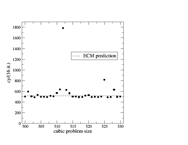
Figure 3: Serial runtime of 16 scalar iterations of version 3 versus problem size (cubic domain). Statistical variations of individual measurements were always below 1%.
Second, the scalar gcc-generated code is still limited by data transfers due to the non-overlapping scalar loads in the core. However, in this case we know that only 15% of the time is spent in main memory data transfers. The best advice here is thus “make the compiler produce better code,” i.e., vectorize and use all available floating-point registers.
To make the analysis complete we should now validate the model by checking the actual data transfers using likwid-perfctr or some other HPM tool. I am skipping this step here; suffice it to say that the validation is successful within the usual accuracy limits of HPM events.
Saturation behavior
The single-core analysis gives us a baseline for the parallel code. While the ECM model yields runtime predictions, scalability is usually studied using a “higher is better” metric such as (in case of stencils) LUP/s. We can easily translate the cycles c for a given number of LUPs W into a performance number:P=\frac{W}{c}\times fThe parallel code is very simple:
#pragma omp parallel for private(ss,s0) reduction(+:gosa) schedule(static)
for(int i=1 ; i<imax-1 ; ++i)
  for(int j=1 ; j<jmax-1 ; ++j)
    for(int k=1 ; k<kmax-1 ; ++k){
      s0 = ...
      ss = ( s0 * a[3][i][j][k] - p[i][j][k] ) * bnd[i][j][k];
      gosa = gosa + ss*ss;
      wrk2[i][j][k] = p[i][j][k] + omega * ss;
    }
At the problem sizes we choose here, the overhead from the OpenMP parallelization is not an issue. Of course we have to make sure now that the compiler can still produce the same loop code, regardless of the OpenMP parallelization. While this is true for the Intel compiler, the gcc 7.2.0 binary runs about 5% slower with one OpenMP thread compared to the version with OpenMP turned off. We could fix this by putting the innermost (two) loop(s) into a separate function, but it doesn’t really make much of a difference.
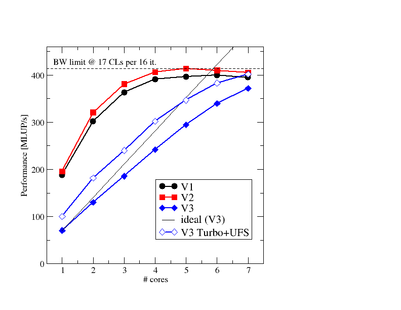
Figure 4: Scaling of all three variants in one ccNUMA domain (problem size 5053). The open diamonds show the scalar code with Turbo mode and Uncore Frequency Scaling turned on.
Figure 4 shows performance scaling data at a problem size of 505^3 for the three variants. First of all, we note that all codes stay within the bandwidth limit set by the broken 3D layer condition (17 cache lines per 16 iterations, dashed line). V1 tops out a little lower, mainly because of the larger amount of concurrent data streams (17 instead of 10 for V2). The general behavior is quite similar, though. The fact that the 3D layer condition gets broken somewhere between 2 and 5 threads is invisible here since other effects are more dominant. Although the ECM model predicts saturation at three cores, we really need one or two more. This is a well-known deficiency of the model near the saturation point, which can be fixed by introducing a bandwidth-dependent latency penalty [4], but that’s something for another post.
The scalar code is interesting: Assuming linear scaling we may expect that even this slow code can saturate the bandwidth, but it fails to do so; of course, a small part of the problem is the layer condition breaking along the way, but mostly it is again excess latency setting in as soon as the bandwidth nears its maximum. However, there is a hardware feature that saves gcc: If we activate Turbo mode and Uncore frequency scaling (UFS), the processor can set its frequency domain as it pleases. This gives us a whopping 40% speedup at one core, and leads to saturation at seven (open diamonds). It burns energy like mad, but gcc’s reputation is redeemed. In essence, if you run the parallel code you may not even notice that the compiler has done a lousy job.
Funny note: I discovered after those experiments that gcc 7.2.0 does vectorize the SIMD-friendly code if I omit the -std=c99 option. Go figure.
Miscellaneous
If you compare the above analysis with the Roofline analyis in my previous post, you will notice that I had used a different memory bandwidth there (about 55 GB/s). This was because the Haswell node ran in non-CoD mode at that time, i.e., with 14 cores per ccNUMA domain. This led to a slightly lower aggregated socket bandwidth compared to the CoD mode used here.
The code for the benchmarks is part of kerncraft. Note that kerncraft is currently (as of version 0.6.7) not able to analyze the layer conditions for SIMD-unfriendly data layout analytically, and the cache simulator has a hard time with a working set of 7 GB. What I did was employ the “ECMCPU” analysis model, which just runs IACA on the compiled code for the in-core modeling. Since the data transfers are the same as for the SIMD-friendly data layout, this was sufficient in this particular case. The very convenient “Benchmark” mode of kerncraft works, though. I have used it to take all the performance measurements. I used a custom machine description file for my machine (for adjusted compiler options and the 43 byte/cy L2 bandwidth). You can download it from here: HaswellEP_GHa_CoD.yml
[1] H. Stengel, J. Treibig, G. Hager, and G. Wellein: Quantifying performance bottlenecks of stencil computations using the Execution-Cache-Memory model. Proc. ICS15, the 29th International Conference on Supercomputing, June 8-11, 2015, Newport Beach, CA. DOI: 10.1145/2751205.2751240. Preprint: arXiv:1410.5010
[2] J. Hofmann, G. Hager, G. Wellein, and D. Fey: An analysis of core- and chip-level architectural features in four generations of Intel server processors. In: J. Kunkel et al. (eds.), High Performance Computing: 32nd International Conference, ISC High Performance 2017, Frankfurt, Germany, June 18-22, 2017, Proceedings, Springer, Cham, LNCS 10266, ISBN 978-3-319-58667-0 (2017), 294-314. DOI: 10.1007/978-3-319-58667-0_16. Preprint: arXiv:1702.07554
[3] J. Hammer, G. Hager, J. Eitzinger, and G. Wellein: Automatic Loop Kernel Analysis and Performance Modeling With Kerncraft. Proc. PMBS15, the 6th International Workshop on Performance Modeling, Benchmarking and Simulation of High Performance Computer Systems, in conjunction with ACM/IEEE Supercomputing 2015 (SC15), November 16, 2015, Austin, TX. DOI: 10.1145/2832087.2832092, Preprint: arXiv:1509.03778
[4] J. Hofmann, G. Hager, and D. Fey: On the accuracy and usefulness of analytic energy models for contemporary multicore processors. In: R. Yokota, M. Weiland, D. Keyes, and C. Trinitis (eds.): High Performance Computing: 33rd International Conference, ISC High Performance 2018, Frankfurt, Germany, June 24-28, 2018, Proceedings, Springer, Cham, LNCS 10876, ISBN 978-3-319-92040-5 (2018), 22-43. DOI: 10.1007/978-3-319-92040-5_2, Preprint: arXiv:1803.01618. Winner of the ISC 2018 Gauss Award.