Georg Hager's Blog

Random thoughts on High Performance Computing

Content

Fooling the masses – Stunt 6: Ignore affinity and topology issues!

AMD Epyc 7451 node

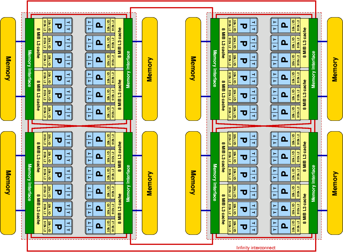
Fig. 1: A dual-socket AMD Epyc 7451 node with four “Zeppelin” dies per socket (eight ccNUMA domains per node). Each 8 MiB L3 cache is shared by three cores, i.e., half the die.

(See the prelude for some general information on what this is all about)

Real scientists are not bothered by details such as multicore, cache groups, ccNUMA, SMT, or network hierarchies. Those are just parts of a vicious plot to take the fun out of computing. Ignoring the associated issues like bandwidth bottlenecks, NUMA locality and contention penalties, file system buffer cache, synchronization overheads, etc., will make them go away.

If you present performance data and people ask specific questions about affinity and topology awareness, answer that it’s the OS’s or the compiler’s job, or the job of some auto-tuning framework, to care about those technicalities. Probably you can show off by proving that your code scales even though you run it without topology awareness; this can be easily achieved by applying Stunt 2 – just slow down code execution enough to make all overheads vanish.

If you run into problems like mysterious performance fluctuations, or performance being too low altogether (a direct but often ignored consequence of applying Stunt 2), blame the system administrators. Being lowly minions of top-achieving scientists like you, they will have the time to figure out what’s wrong with their hardware. If they tell you it’s all your fault, send a scathing e-mail to their boss and cc: your university president or company CTO, just for good measure. Finally, if all else fails, publish a paper at a high-profile conference stating that the hardware of manufacturer X shows horrible performance, especially together with compiler Y and library Z, and that the cluster you had access to was too small to get the results that you wanted in time. That’s why you are about to write a generous research proposal for a federal supercomputing facility. Anything less just won’t cut the mustard!


Fooling the masses – Stunt 5: Instead of performance, plot absolute runtime versus CPU count!

(See the prelude for some general information about what this is all about)

Runtime versus CPU count

Fig. 1: If you plot the program’s runtime versus CPU count at strong scaling, nobody will be able to tell whether scalability is good or bad at the larger CPU counts.

Apart from using a logarithmic scale (see Stunt 3), deficiencies in scalability can also be hidden effectively by plotting absolute runtime. This works for strong scaling only, since weak scaling shows constant or increasing runtime when the number of CPUs goes up.

Of course you should start at a very low number of CPUs (and not use log scale this time, or you’ll be caught immediately). Then, runtimes at large CPU counts will be compressed to a small ordinate range, and nobody will be able to tell the difference between a 1.5 or a 2.0 speedup — just as you need it (see Fig. 1). The casual observer is always stunned by the strong decrease in runtime, without noticing its insignificance. Even if the curve starts turning upward at some critical CPU count, you can often get away with the statement that your code scales up to this point, even though parallel efficiency has gone down the drain much sooner.

Excel eye candy obfuscation fury

Fig. 2: A little 3D and texture sugar will hide unpleasant truths even better. And yes, the numbers are very different at large CPU counts!

To make the results even more striking you can use the CPU time per core instead of overall wallclock time. Depending on how you determine CPU time, overhead like OS calls (system time) may be omitted and you get better-looking results. Not that it would matter in any way, because it’s all swamped by the scale.

A very popular variant of runtime graphs is the “obfuscation by eye candy fury”. Excel makes it so easy to add visual sugar to your graphs; you can literally click your audience into oblivion: 3D beveled columns, drop shadows, fill gradients on walls (and columns!), fancy textures, etc. etc.  A large number of data sets will also help (but see Stunt 11 for the full potential). Combined with the runtime-vs-CPU-count trick from above, comparing different systems without revealing the truth is a solved problem (see Fig. 2). Don’t forget to choose colors that will be indistinguishable in a grayscale printout; readers can’t criticize what they can’t see…

Fooling the masses – Stunt 4: Quietly employ weak scaling to show off!

(See the prelude for some general information about what this is all about)

As we have seen in Stunt 2 about slowing down code execution, making all parts in the speedup formula except communication overhead more dominant is good for the straightness of your scalability graph. Weak scaling, i.e., keeping the problem size per worker constant while increasing the number of workers, is probably the simplest way to achieve this (\alpha=1 in the speedup formula). Neglecting boundary effects, many codes will then show a constant ratio of communication overhead versus computation time; given a reasonably nonblocking network hierarchy, linear scalability often comes for free, at least for a large enough number of nodes. A positive side effect is that you don’t even have to recompile, let alone change your code.You can then even show real performance numbers, not just speedups!

Fig. 1: Weak scaling with a dominating serial part. The scalability function has a small slope, but the “work” done in the parallel part scales perfectly.

In case there is no communication problem but a large serial part, just by choosing the right metric to look at you can get perfect scaling, i.e., S(N)=N. Here’s how it works: Let’s assume that, despite weak scaling, your code is dominated by a sequential part. Hence, it’s S(N)=s+(1-s)N. The function is linear but has a small slope, which doesn’t look good and leads to a parallel efficiency \varepsilon(N)=S(N)/N that is much smaller than 1. However, looking at how the processors spend their time it is clear that the speedup function for the  purely parallel work per time unit, i.e., not counting any overhead, is linear in N with a slope of 1  (see Fig. 1). How can this be used to polish performance numbers? Just report a performance metric that is valid only for the purely parallel part of the application! MFlop/s or MLup/s (lattice site updates) will do fine, for instance. If the “overhead” part contains no lattice updates, the MLup/s metric has a perfect speedup function S_\mathrm{mlups}(N)=N, the performance graph is linear with no y-intercept, and \varepsilon(N)=1, even though all but one processor are twiddling their thumbs most of the time. Problem solved. Stay tuned for Stunt 10, where we will show that a similar trick is possible for communication-dominated cases as well.

The reason why it works is that we have chosen a different notion of what “work” means in the speedup formula. Speedup is defined as

S(N)=\frac{\text{work/time with \textit{N} workers}}{\text{work/time with 1 worker}}~,

no matter whether the amount of work varies with N or not. While there is no discussion about what “time” means, we can give different meanings to “work”. If “work” is chosen so that only operations in the parallel part are counted, parallel efficiency is perfect at weak scaling (\alpha=1). That trick cannot be pulled at strong scaling, though (it is left to the reader to prove this…).

It is certainly advisable to omit any mention of the fact that weak scaling was used. Your audience will cheer and rejoice in the light of such straight lines! However, don’t let them watch too long or they’ll ask nasty questions…

This stunt is essentially #4 of Bailey’s original “Twelve ways to fool the masses.”

Fooling the masses – Stunt 3: The log scale is your friend!

(See the prelude for some general information about what this is all about)

Sometimes a data plot just isn’t straight enough. You know that your code scales, but the bloody cluster stubbornly ignores this fact and the performance graph looks like a skew-whiff banana:

How are you supposed to drive your point home? Do not despair! Help is on the way. We’ll be guided by the Great Old Ones and just use a log scale. Whether it’s lin-log, log-lin, or log-log should be determined according to your particular needs for obfuscation. The point is that a log scale tends to underemphasize deviations between graphs in the same plot. Here we have chosen the log-log variant:

Doesn’t this look much nicer? You can easily attach the “almost linear scaling” label to it, although parallel efficiency is barely above 60% at the largest number of workers.

Fooling the masses – Stunt 2: Slow down code execution!

(See the prelude for some general information about what this is all about)

Common sense dictates that whenever you speed up any part of an application, be it computation, communication, or I/O, time to solution must go down. Why should one then try to slow down computations? In a sense, this stunt is similar to Stunt 1, but there’s more to it: Whenever there is some parallel overhead that adds to pure code execution time, the denominator in our “speedup” formula from Stunt 1 gets larger, impeding scalability. To make the discussion more general, let’s look at the speedup for parallel execution with N workers and a sequential part s, and scale the parallel problem size with a factor proportional to N^\alpha:

\large S(N)=\frac{s+(1-s)N^\alpha}{s+(1-s)N^{\alpha-1}+c_\alpha(N)}

Here, c_\alpha(N) contains all the overhead that is not directly related to code execution: Communication, I/O, synchronization, etc. The parameter \alpha can be used to set the problem size scaling: \alpha=0 for strong scaling, \alpha=1 for weak scaling. Now if the “computation” parts of this expression, i.e., everything except c_\alpha(N), get larger (e.g., by a factor of \mu>1), the impact of overhead goes down by just this factor:

\large S_\mu(N)=\frac{\mu(s+(1-s)N^\alpha)}{\mu(s+(1-s)N^{\alpha-1})+c_\alpha(N)}=\frac{s+(1-s)N^\alpha}{s+(1-s)N^{\alpha-1}+\color{red}{c_\alpha(N)\mu^{-1}}}

In layman’s terms, this effect can be summarized as “A slow machine scales better,” and it is one of the key reasons why Stunt 1 works.

Three corollaries immediately follow from this:

  1. Do not use high compiler optimization levels or the latest compiler versions. This is always possible if the machine you use just isn’t slow enough.
  2. Use a convoluted C++ framework that hides all performance complexities by neatly overloaded operators and template mechanics. You can then claim that, since the compiler will generate “optimal” code, performance is not your concern any more.
  3. If scalability is still bad, parallelize some short loops with OpenMP. That way you can get some extra bonus for a scalable hybrid code! Everyone knows today that “one should go hybrid”, even if there’s no indication that this will do any good.

If someone asks for time to solution, answer that if you had a bigger machine, you could get the solution as fast as you want. This is of course due to the superior scalability of your code!

However, let’s not forget that there are valid arguments for machines with slow processors like the (now extinct) IBM Blue Gene. Apart from the power consumption issue (a core that is \mu times slower than a standard x86 core consumes far less than 1/\mu times the power), it can be beneficial to use \mu N slow CPUs instead of N fast ones, if communication overhead has a certain dependence on N. See our book for a theoretical treatment of “slow computing”.

Fooling the masses – Stunt 1: Report speedup, not absolute performance!

(See the prelude for some general information about what this is all about.)

Have you ever been stuck with a slow machine, but needed to compare it with something else (much faster) you didn’t have the wits or guts to use? Or even worse, you want to sell one of those slow machines and no matter what you do, you just can’t get your codes run faster than your competition? This stunt may be for you. On a very simple level, if we define “speedup” as

\large S(N)=\frac{\text{work/time with \textit{N} workers}}{\text{work/time with 1 worker}}

it is clear that it is a gift from heaven: If S\approx N we speak of “good scalability”, but there is no indication of how fast a certain problem can be solved, or even how many “operations” per time unit are performed. Note that the speedup definition above works for strong and weak scaling scenarios alike.

Stunt 1 - Performance vs. speedup

In this example we see a comparison between some “big iron” machine, let’s call it “NEC”, and a standard cluster, which you would like to show off in your presentation. As you can see on the left, the big machine outperforms the cluster by far on a worker-by-worker basis; however, if the one-worker performance is normalized to one we see that the cluster “scales better”. Whatever the particular reasons for this may be, presenting scalability (or speedup) instead of absolute performance is key.

Certainly, not all audiences are so easily deceived, but labeling your talk with the word “executive” somewhere in the title will fend off the geeks and leave you with a convenient flock of suits who will eat what you give them.

Fooling the masses with performance results on parallel computers – prelude

In 1991, David H. Bailey published his insightful “Twelve Ways to Fool the Masses When Giving Performance Results on Parallel Computers.” In that humorous article, Bailey pinpointed typical “evade and disguise” techniques for presenting mediocre performance results in the best possible light. These are the original 12 ways:

  1. Quote only 32-bit performance results, not 64-bit results.
  2. Present performance figures for an inner kernel, and then represent these figures as the performance of the entire application.
  3. Quietly employ assembly code and other low-level language constructs.
  4. Scale up the problem size with the number of processors, but omit any mention of this fact.
  5. Quote performance results projected to a full system.
  6. Compare your results against scalar, unoptimized code on Crays.
  7. When direct run time comparisons are required, compare with an old code on an obsolete system.
  8. If MFLOPS rates must be quoted, base the operation count on the parallel implementation, not on the best sequential implementation.
  9. Quote performance in terms of processor utilization, parallel speedups or MFLOPS per dollar.
  10. Mutilate the algorithm used in the parallel implementation to match the architecture.
  11. Measure parallel run times on a dedicated system, but measure conventional run times in a busy environment.
  12. If all else fails, show pretty pictures and animated videos, and don’t talk about performance.

There are further explanations in the original paper for each item.

After two decades, it’s high time for an update. In 1991 the supercomputing landscape was governed by the “chicken vs. oxen” debate: The famous question “If you were plowing a field, which would you rather use?… Two strong oxen or 1024 chickens?” is attributed to Seymour Cray who couldn’t have said it better. Cray’s machines were certainly dominating in the oxen department, but competition from massively parallel systems like the Connection Machine was building up. At that time, users were much more used to dive into system-specific optimizations — with no MPI and OpenMP standards, portability of parallel programs was pretty much restricted to a certain vendor. And the use of double precision floating point was probably not as much a matter of course as it is today.

In the past two decades, hybrid, hierarchical systems, multi-core processors, accelerator technology, and the dominating presence of commodity hardware have reshaped the landscape of High Performance Computing. It’s also not so much oxen vs. chickens anymore; ants have received more than their share of hype. However, some things never change. My points (which I prefer to call “stunts”) are derived from Bailey’s original collection, and some are identical or merely reformulated. Others are new, reflecting today’s boundary conditions.

Although these musings are certainly inspired by experience with many publications and talks in HPC, I wish to point out that (i) no offense is intended, (ii) I am not immune to the inherent temptations myself and (iii) this all still just meant to be fun.

This is the list of stunts. It will be extended along the way:

  1. Report speedup instead of absolute performance!
  2. Slow down code execution!
  3. The log scale is your friend!
  4. Quietly employ weak scaling to show off!
  5. Instead of performance, plot absolute runtime versus CPU count!
  6. Ignore affinity and topology issues! 
  7. Be creative when comparing scaled performance!
  8. Impress your audience with awe-inspiring accuracy!
  9. Boast massive speedups with accelerators!
  10. Always emphasize the “interesting” part of your work!
  11. Show data! Plenty. And then some.
  12. Redefine “performance” to suit your needs!
  13. If they get you cornered, blame it all on OS jitter!
  14. Secretly use fancy hardware setups and software tricks!
  15. Play mysterious!
  16. Worship the God of Automation!